
You shipped a vision-language model on the same GPU stack that served your text LLM. Same vLLM config, similar parameter count, no red alarms in monitoring – yet throughput fell anyway. Inter-token latency crept up. Batch-size tuning helped a little; quantisation helped a little; neither explained the gap.
The issue is not a bad deploy. The issue is that multimodal inference is secretly two completely different workloads with opposite hardware appetites, and you are running both on one piece of silicon. Aggregate GPU utilisation looks fine because each phase is idle during the other one’s bottleneck. Users feel the slowdown; your dashboard hides it.
Encode vs Decode: A Resource Inversion
A VLM pipeline is two engines operating in sequence. Understanding the difference between them is the whole article, so let us be precise.
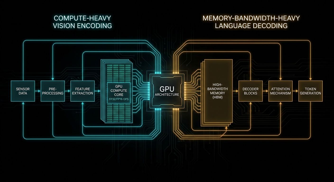
Image encoding is a matrix-intensive operation. Patches from the image flow through a ViT-style vision tower; the bottleneck is floating-point compute. Profiling on consumer cards typically shows 80%+ tensor-core utilisation with single-digit HBM bandwidth use. The GPU is doing arithmetic; it is barely touching main memory.
Token decoding is the exact opposite. Each new token requires reloading the full weight matrix and the growing KV cache from HBM, performing a small amount of arithmetic, emitting one token, and repeating. On datacenter GPUs, bandwidth saturates while tensor cores sit nearly idle. The GPU is reading memory; it is barely doing arithmetic.
Co-locate both phases on one card and you permanently pay for capacity that each phase ignores. During encode, HBM is underused. During decode, tensor cores are underused. Neither phase gets hardware tuned for what it actually needs.
“Multimodal large language model (MLLM) inference splits into two phases with opposing hardware demands: vision encoding is compute-bound, while language generation is memory-bandwidth-bound.” — Donglin Yu et al., arXiv:2603.12707
Kleppmann’s Designing Data-Intensive Applications makes a related point about aggregate metrics: when the bottleneck shifts between pipeline stages, a single utilisation number averages two opposite stories into one misleadingly healthy reading. You need phase-level instrumentation, not a system-wide gauge.
Visual Tokens and the KV Cache Problem
To understand why high-resolution images hurt decode performance specifically, you need to understand what the KV cache holds and why it costs bandwidth.
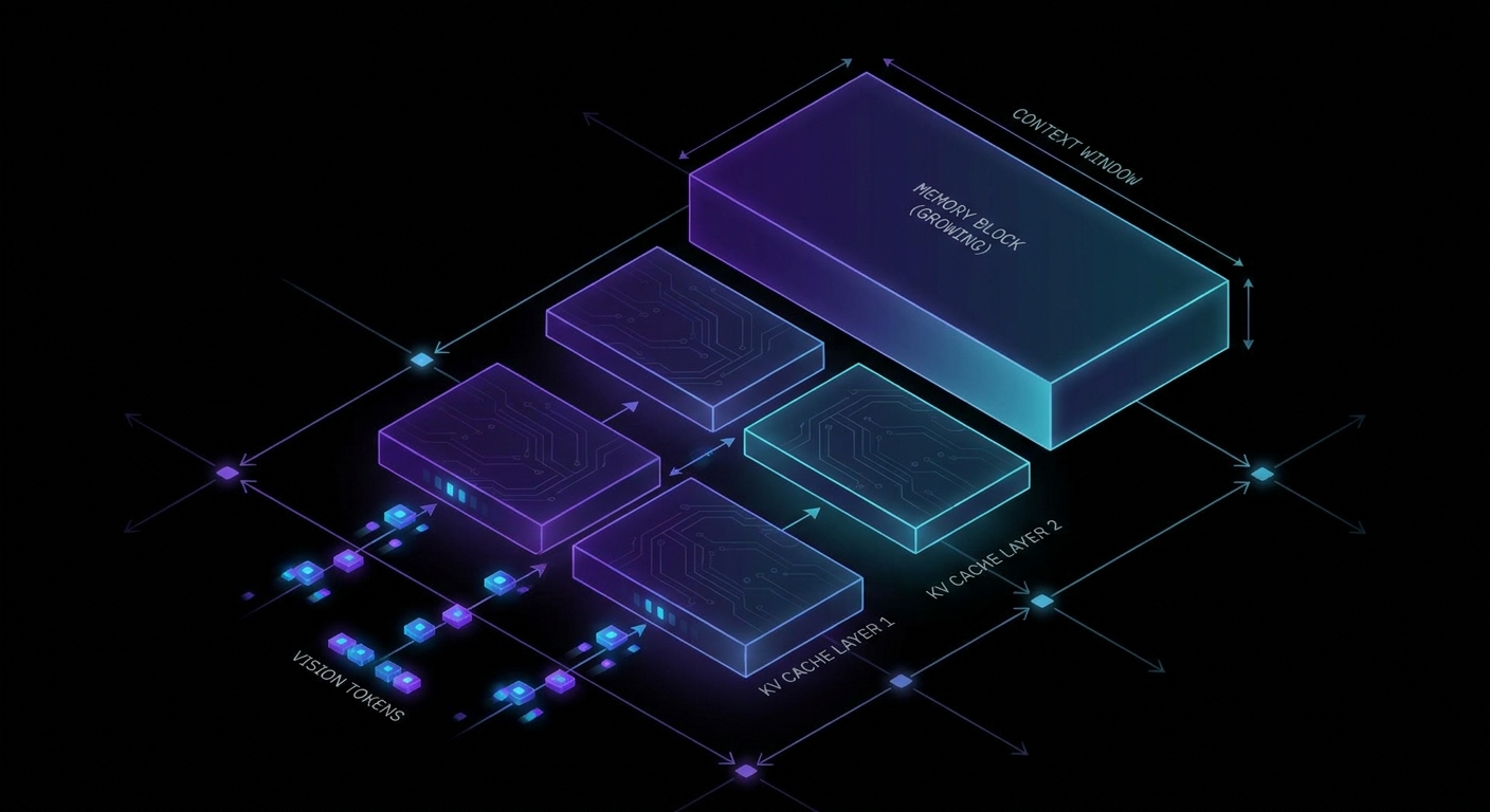
During prefill, the model builds a KV cache: per-layer key and value tensors for every token in the input context. Without it, autoregressive decode would recompute full attention over the entire history on each step, which scales quadratically with sequence length. The cache trades memory for compute. That is a good trade – unless the cache is enormous.
Visual tokens join the cache at prefill and stay there for every single decode step. The model has already compressed the image into embeddings, but hundreds of image tokens still occupy HBM and get re-read with every token generated. The bandwidth cost is proportional to output length, not to how “done” the image processing feels.
Case 1: High-Resolution Inputs Bloat the Cache Before Decode Begins
A modest 336×336 image can produce approximately 576 visual tokens. Add 128 text tokens and you have 704 tokens in the KV cache before the first answer token is generated. For a 7B MHA model at FP16, that is roughly 350 MB per request. Scale to eight concurrent requests and you are using ~2.8 GB of cache capacity before generation has even started.
// FP16 KV cache size (one sequence):
// bytes ≈ 2 × layers × seq_len × kv_heads × head_dim × 2
//
// Text-only request (128 tokens):  ~64 MB
// Same request + one image (704 tokens): ~350 MB
//
// Quantisation reduces bytes per element.
// It does not remove the 576 persistent image token slots
// that get re-read on every decode step.
Case 2: Concurrency Makes the Problem Super-Linear
Raising batch size under multimodal load can actually hurt. More concurrent requests means more fat KV caches competing for the same HBM bandwidth simultaneously. Inter-token latency often climbs faster than image-token count alone would predict – the slope steepens because bandwidth contention compounds.
// Metrics to correlate (log all three together):
// - kv_cache_bytes per request vs image resolution
// - hbm_bandwidth_util during decode phase only
// - itl_p95 vs concurrent_request_count
//
// If ITL grows super-linearly with concurrency, you have
// bandwidth contention, not a "slow model".
Where to Split the Pipeline
Once you accept that the two phases want different hardware, the next question is where to draw the boundary – and the answer matters more than it looks.
Prefill/decode split cuts the pipeline after prefill: a prefill node builds the KV cache and ships it to a decode node. The payload is the full KV tensor – hundreds of MB to GB depending on model depth and context length. That demands high-bandwidth interconnect (NVLink, InfiniBand). Ordinary PCIe clusters do not have enough throughput to make this worthwhile.
Encoder/decoder split cuts earlier: a vision encoder node processes the image and ships only the resulting embeddings to the LLM node. The payload is just token_count × hidden_size – the KV cache does not exist yet, so you never ship it across the wire.
// LLaVA-7B-style numbers (576 vision tokens, dim 4096, FP16):
//
// Vision embeddings across the wire: ~4.5 MB
// Full KV cache for same context: ~350 MB
// Ratio: ~78x less data at the encoder boundary
//
// PCIe transfer at 16 GB/s:
//   4.5 MB  -> sub-millisecond
//   350 MB  -> tens of milliseconds
“Partitioning here reduces transfer complexity from O(L * s_ctx) bytes (GB-scale KV caches under stage-level disaggregation) to O(N_v * d) bytes (MB-scale embeddings), an O(L) reduction where L is the transformer depth.” — Donglin Yu et al., arXiv:2603.12707
Yu et al. report 12×–196× transfer reductions across current architectures depending on model depth. The gap widens as models get deeper: embeddings stay compact at roughly the same size, while KV migration cost grows linearly with the number of transformer layers.
Matching Silicon to Phase
Once the split is in place, hardware assignment follows naturally. Encode nodes want FLOPs-per-dollar – consumer or commodity compute cards work well here. Decode nodes want HBM bandwidth and large VRAM – A100/H100 class. An RTX 4090 and an A100 have similar peak TFLOPS; the 4090 wins on FLOPs per dollar, but the A100 wins on memory bandwidth and total VRAM.
Heterogeneous deployments under this split have shown approximately 40% cost savings versus homogeneous baselines in recent benchmarks, with no measurable latency regression when scheduling is handled correctly. The standard inference engine tricks – CUDA graphs, packed prefill, paged KV – still apply and still matter, but they do not substitute for matching silicon to the workload phase.
Case 3: Text-Only Traffic Leaves Encoders Idle
A hard encode/decode split creates a utilisation problem during text-only bursts: the encoder pool sits idle while the decoder pool is saturated. Work-stealing schedulers solve this by letting encoder nodes absorb decode jobs when the vision queue is empty. The roles are not symmetric – decode workers cannot encode – but encode workers can handle text-only generation with their available compute, recovering utilisation without fragile dynamic role reassignment.
Diagnose Before You Re-Architect
Before splitting pools, confirm the bottleneck is actually the encode/decode phase mismatch and not something simpler:
- Isolate the variable. Hold model and sampling parameters fixed; vary only image resolution and count across requests.
- Plot ITL against vision-token count at a realistic concurrency level. A flat slope means bandwidth is not the issue.
- Profile each phase separately using Nsight Systems or equivalent. Look for compute-bound encode and bandwidth-bound decode as the diagnostic signature.
- Correlate with your serving metrics. vLLM exposes KV-cache utilisation and scheduler queue depth; use them.
When Monolithic Serving Is Enough
Dual pools make economic sense at sustained multimodal volume where a significant fraction of total inference spend is attributable to this mismatch – roughly a third or more of your bill. For prototypes, low-QPS applications, and teams that do not have the operational capacity to run and schedule heterogeneous fleets, staying on a single GPU is the right call until the numbers force a change. The same encode/decode asymmetry applies to audio and video input towers, not just vision – so if you later add speech input, the analysis carries over directly.
What to Check Right Now
- KV bytes per request across the range of image resolutions your users actually send.
- Phase-split profiling to confirm compute-bound encode and bandwidth-bound decode are both present.
- ITL slope under concurrent load – super-linear growth signals bandwidth contention, not raw model speed.
- Business case first. Heterogeneous pools add scheduling complexity. Run the cost arithmetic before committing to the architecture.
Half your GPU was on holiday during every request. The fix is giving each phase the silicon it actually uses – and knowing, precisely, which phase is slowing you down before you spend money on a bigger card.
nJoy 😉