

How to Read AI Leaderboards in 2026 Without Getting Played
Model launches now ship with a chart before they ship with a changelog. Artificial Analysis Intelligence Index here, Chatbot Arena score there, SWE-bench percentage in...
Jul 24, 2026Deep technical writing on AI, LLMs, and Linux. 474+ articles. 3 structured courses. 100% free.
Model launches now ship with a chart before they ship with a changelog. Artificial Analysis Intelligence Index here, Chatbot Arena score there, SWE-bench percentage in...
Jul 24, 2026
Microsoft Build 2026 was billed as an agentic platform story. Underneath the keynotes sits a sharper move: seven in-house MAI models, led by MAI-Thinking-1 for...
Jul 24, 2026
Cohere’s pitch for years was enterprise NLP you could run inside your boundary. With Command A+, released May 2026, they consolidate reasoning, multimodal document work,...
Jul 24, 2026
Every board deck now mentions AI agents. Most organisations still cannot put one into production on a billing queue, a claims line, or an IT...
Jul 24, 2026
July 2026 is the month open MoE stops being a niche hobby. Kimi K3 (2.8T MoE, weights promised by 27 July), DeepSeek V4 (MIT weights...
Jul 24, 2026
DeepSeek V4 is not waiting for you to notice. The API docs already expose deepseek-v4-pro and deepseek-v4-flash with 1M context, flat USD pricing, and a...
Jul 24, 2026
Meta’s Muse Spark 1.1 release is not just a model bump. It pairs a multimodal agentic model with the first public preview of the Meta...
Jul 24, 2026
Grok 4.5 lands with a story that is easy to misread. The headline is not “another frontier model” but “a coding model trained with your...
Jul 24, 2026The AI scene from the C-level. Strategic briefings for executives who need the point, not the hype.
Every board deck now mentions AI agents. Most organisations still cannot put one into production on a billing queue, a claims line, or an IT...
Jul 24, 2026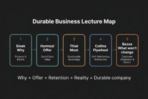
Alex Hormozi sat with Steven Bartlett for nearly two and a half hours. Most clips will sell you three minutes of “reality is the moat.”...
Jul 20, 2026
By 2026 every competitor has access to the same models. The returns go to the companies that can absorb machine intelligence into how they actually...
Jul 3, 2026In-depth dives on frontier lab releases, eval metrics, and infra moves - claim-audited, not press-release remixes.
Model launches now ship with a chart before they ship with a changelog. Artificial Analysis Intelligence Index here, Chatbot Arena score there, SWE-bench percentage in...
Jul 24, 2026
Microsoft Build 2026 was billed as an agentic platform story. Underneath the keynotes sits a sharper move: seven in-house MAI models, led by MAI-Thinking-1 for...
Jul 24, 2026
Cohere’s pitch for years was enterprise NLP you could run inside your boundary. With Command A+, released May 2026, they consolidate reasoning, multimodal document work,...
Jul 24, 2026
Every board deck now mentions AI agents. Most organisations still cannot put one into production on a billing queue, a claims line, or an IT...
Jul 24, 2026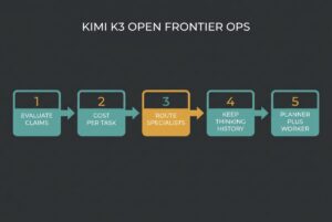
The loudest take on Moonshot’s Kimi K3 is that open weights just “crushed” every closed frontier model. That is marketing...
Jul 24, 2026
Your RAG benchmark says the system is excellent. The benchmark may also be the least trustworthy component in the stack....
Jul 21, 2026
The hard part of AI coding is no longer typing. It is keeping thirty half-finished agent sessions in your head...
Jul 18, 2026
DeepSeek has a habit of publishing the things other labs treat as trade secrets. Their latest release, DSpark, is a...
Jul 3, 2026
FFmpeg is what happens when a Swiss Army knife gets a PhD in multimedia and then refuses to use a...

WordPress ships slow. Not broken-slow, but “a friend who takes 4 seconds to answer a yes/no question” slow. The default...

Redis is one of those tools you adopt on a Monday and depend on completely by Thursday. It’s fast, it’s...
For nmap to even make a guess, nmap needs to find at least 1 open and 1 closed port on...