DSpark Explained: How DeepSeek Made LLM Serving 60-85% Faster Without Losing a Single Token of Quality

DeepSeek has a habit of publishing the things other labs treat as trade secrets. Their latest release, DSpark, is a speculative decoding system that made per-user generation 60–85% faster in production and kept serving tiers alive that their old system simply could not reach, all with zero loss in output quality. The paper is dense, the ideas are genuinely clever, and most coverage of it stops at the headline numbers. This page is the opposite: a step-by-step instruction guide that builds the whole system up from first principles, with the actual numbers from the paper, the failure modes that motivated each design decision, and the commands to run the open-source code yourself. If you can follow a for-loop, you can follow this.

What You Will Learn

This guide covers the complete DSpark stack, in the order you need to understand it:

• Step 1 — why autoregressive generation is slow, and why the bottleneck is memory bandwidth, not arithmetic
• Step 2 — how speculative decoding works, and why it is mathematically lossless
• Step 3 — the drafter dilemma: autoregressive drafters vs parallel drafters, and the suffix decay problem
• Step 4 — DSpark fix number one: the semi-autoregressive architecture with a Markov head
• Step 5 — DSpark fix number two: the confidence head and calibration
• Step 6 — DSpark fix number three: the hardware-aware prefix scheduler
• Step 7 — the production results, with the honest caveats the paper itself gives
• Step 8 — how to run the open-source DeepSpec code yourself

Everything here is sourced from the DSpark paper (“DSpark: Confidence-Scheduled Speculative Decoding with Semi-Autoregressive Generation”, DeepSeek-AI and Peking University) and the DeepSpec repository. Where the paper’s numbers differ from popular summaries, the paper wins.

Paper and Code

All the primary sources, in one place:

• The DSpark paper (PDF) — DSpark: Confidence-Scheduled Speculative Decoding with Semi-Autoregressive Generation, published directly in the DeepSpec repository
• The codebase — deepseek-ai/DeepSpec on GitHub, MIT-licensed full training and evaluation stack for DSpark, DFlash and Eagle3 drafters
• DSpark inside DeepSeek-V4 — deepseek-ai/DeepSeek-V4-Pro-DSpark on Hugging Face, the V4-Pro checkpoint with the DSpark drafting module attached
• Standalone DSpark checkpoints — for example dspark_qwen3_4b_block7; the full checkpoint table (Qwen3-4B/8B/14B and Gemma-4-12B targets, all three algorithms) is in the DeepSpec README
• The DeepSeek-V4 technical report — DeepSeek-V4: Towards Highly Efficient Million-Token Context Intelligence (arXiv 2606.19348), covering the serving system DSpark was deployed into

Step 1 — Understand Why Generation Is Slow

A large language model generates text autoregressively: one token per forward pass, each pass conditioned on everything generated so far. That single sentence explains most of the latency you experience with any chat model. A 2,000-token answer requires 2,000 sequential forward passes, and pass number 1,999 cannot start until pass number 1,998 has finished. Latency grows linearly with output length, full stop.

The counter-intuitive part is where the time goes. It is not the arithmetic. Modern GPUs are monstrously good at matrix multiplication; pushing one token’s worth of activations through even a huge model is a small burst of work. The expensive part is fetching the model’s weights and the KV cache (the stored attention states of every previous token) from GPU memory into the compute units, for every single token generated. During single-token decoding the GPU spends most of its time waiting on memory, not computing. In roofline-model terms, decode is memory-bandwidth-bound, not compute-bound. This is exactly the kind of hardware sympathy that Kleppmann’s “Designing Data-Intensive Applications” preaches for databases: know whether you are bound by compute, memory, or I/O before you optimise anything.

Here is the failure written as code, because it makes the fix obvious later:

Case 1: The Memory-Bandwidth Wall

The naive decode loop pays the full memory-fetch cost per token and cannot parallelise across output positions:

# Naive autoregressive decoding
tokens = prompt_tokens
while not finished:
    # ONE forward pass = stream ALL model weights + KV cache
    # through the GPU's memory bus, to produce ONE token
    logits = model.forward(tokens)          # memory-bound, GPU mostly idle
    next_token = sample(logits[-1])
    tokens.append(next_token)               # and now do it all again

# 2,000 output tokens = 2,000 full weight streams.
# The FLOPs are cheap. The memory traffic is the bill.

The key observation: if the GPU is going to stream the weights through anyway, verifying eight candidate tokens in one pass costs barely more than verifying one, because the weight traffic dominates and it is shared across the batch of positions. The hardware is begging for parallel work. Autoregressive generation refuses to provide it. Speculative decoding is the trick that provides it.

Step 2 — Speculative Decoding, and Why It Is Lossless

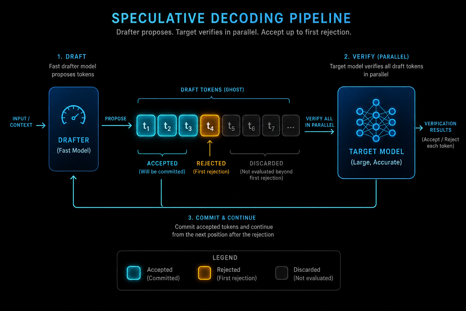
Speculative decoding, introduced independently by Leviathan et al. and Chen et al. in 2023, splits generation into two roles. A small, fast draft model proposes a block of candidate tokens (say 5 to 10). The big, slow target model then verifies the whole block in a single forward pass, which, per Step 1, it can do almost for free. The popular analogy is an intern drafting text and a slow, expensive boss reviewing it with a red pen; the analogy is fine as far as it goes, but the mechanism underneath is worth knowing precisely.

Verification uses rejection sampling. For each draft position, the target model computes its own probability for the drafted token and compares it with the draft model’s probability. Tokens are accepted left to right; the first rejection discards that token and everything after it, and the target model’s own distribution supplies a corrected token at the rejection point. One extra “bonus” token is appended on a fully accepted block. The remarkable property is that this acceptance rule reproduces the target model’s output distribution exactly. Not approximately. The maths guarantees that the stream of tokens you get is statistically indistinguishable from the target model decoding alone.

“Because verification is parallel and the acceptance rule preserves the target distribution exactly, speculative decoding accelerates generation without any quality loss.” — DeepSeek-AI, DSpark paper, Section 1

In pseudocode, one decoding cycle looks like this:

# One speculative decoding cycle
draft = draft_model.propose(context, k=8)        # cheap, fast
p_target = target_model.forward_parallel(context + draft)  # ONE pass

accepted = []
for i, tok in enumerate(draft):
    # accept tok with probability min(1, p_target(tok) / p_draft(tok))
    if accept(tok, p_target[i], p_draft[i]):
        accepted.append(tok)
    else:
        # first rejection: resample from the corrected residual
        # distribution and DISCARD everything after position i
        accepted.append(resample_corrected(p_target[i], p_draft[i]))
        break
else:
    accepted.append(sample(p_target[k]))          # bonus token

context += accepted   # commit, then start the next cycle

The economics are simple: if the target model accepts an average of 4 tokens per verification pass, you have roughly quartered your sequential passes. The whole game is therefore maximising the accepted length per cycle while keeping the drafting itself cheap. Which brings us to the dilemma that DSpark was built to resolve.

Step 3 — The Drafter Dilemma

There are two families of draft model, and before DSpark each was broken in its own way.

Autoregressive drafters (Eagle-style) generate the draft one token at a time, each position conditioned on the previous ones. Draft quality is high because every token knows its actual predecessor. But drafting latency grows linearly with block size, which forces short blocks and shallow drafter architectures. You get coherent drafts that are too short to deliver big speedups.

Parallel drafters (DFlash-style) produce all draft positions in a single forward pass. Drafting latency is nearly independent of block size, so long blocks are cheap. But each position is predicted independently, without knowing what the other positions actually sampled. That independence causes a specific, nameable failure:

Case 2: Suffix Decay, or the “of problem” Problem

When the context admits multiple plausible continuations, a parallel drafter can stitch together fragments of different valid answers. The paper’s own example: the model wants to agree with the user, and both “of course” and “no problem” are valid. Each position marginalises over all possible predecessors instead of conditioning on the one actually sampled:

# Parallel drafter, predicting positions 1 and 2 SIMULTANEOUSLY
# Context: assistant is about to agree with the user.
#
# Position 1 distribution:  {"of": 0.5, "no": 0.5}
# Position 2 distribution:  {"course": 0.5, "problem": 0.5}
#
# Position 2 does NOT know what position 1 sampled.
# All four combinations are possible:
#   "of course"   OK
#   "no problem"  OK
#   "of problem"  incoherent   <-- multi-modal collision
#   "no course"   incoherent   <-- multi-modal collision
#
# 50% of drafts are garbage from position 2 onward.

Two tokens in, half the probability mass is already incoherent. Stretch the block to 8 or 16 tokens and the errors compound: the first few positions are usually fine, and the tail is usually rubbish. The acceptance rate decays rapidly along the block, which is why this is called suffix decay. Every rejected suffix token wasted draft compute to generate and, much worse, wasted target-model batch capacity to verify.

So the dilemma: careful-but-slow, or fast-but-wrong. The industry mostly picked one poison per deployment and lived with it. DeepSeek decided the dichotomy was false.

Step 4 — Fix One: Semi-Autoregressive Generation (the Markov Head)

DSpark keeps the expensive part of the drafter fully parallel and adds a tiny sequential module on top. The paper calls the combination semi-autoregressive. The division of labour:

• Parallel stage. A parallel backbone (DeepSeek’s instantiation builds on DFlash) runs one forward pass over the whole block and produces hidden states and base logits for every position. This is where nearly all the drafter’s compute lives, and it stays O(1) in block length.
• Sequential stage. A lightweight head then sweeps left to right, adding a transition bias to each position’s base logits, conditioned on the token actually sampled at the previous position. The block distribution becomes a proper autoregressive factorisation, so position 2 finally knows what position 1 said.

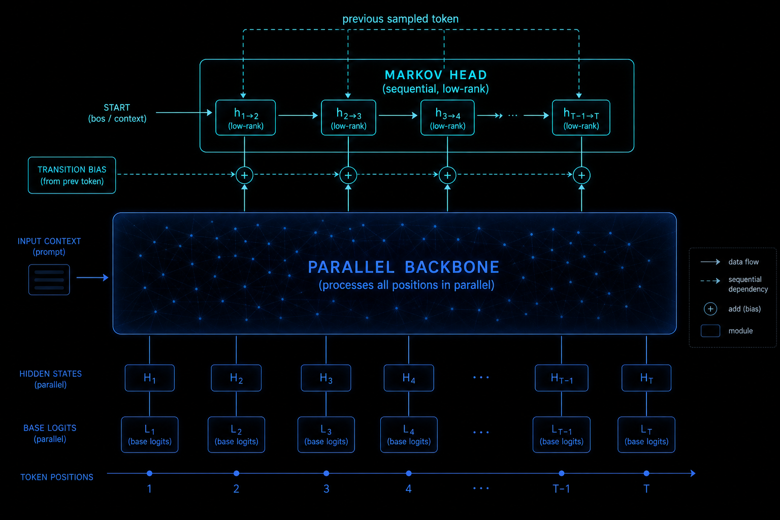
The default sequential module is the Markov head, named after the Markov property in probability theory: the next state depends only on the current state. In principle the transition bias is a full vocabulary-by-vocabulary matrix (for a 100k vocabulary, that is 10 billion entries, absurd). DSpark approximates it with a low-rank factorisation: two thin matrices W1 and W2 with rank r = 256 by default. W1 acts as an embedding lookup for the previous token; W2 projects back to vocabulary logits:

# Markov head: first-order transition bias, low-rank factorised
# W1: [vocab_size, 256]   embedding lookup
# W2: [256, vocab_size]   logit projection

def sequential_stage(base_logits, anchor_token):
    draft = []
    prev = anchor_token
    for k in range(block_size):
        bias = W1[prev] @ W2               # [vocab_size], tiny matmul
        logits_k = base_logits[k] + bias   # nudge, don't overwrite
        tok = sample(softmax(logits_k))
        draft.append(tok)
        prev = tok                          # position k+1 now knows position k
    return draft

# After position 1 samples "of", the bias boosts "course"
# and suppresses "problem" at position 2. Collision avoided.

Note what the head does and does not do. It does not replace the backbone’s predictions; it nudges them with local transition information. The loop is sequential, but each step is a 256-dimensional lookup and projection, which is nothing next to the backbone’s transformer layers. The paper also describes an RNN head variant that carries a gated recurrent state across the whole block prefix rather than just one token back. It helps slightly at long block lengths, but DeepSeek ships the Markov head as the default because the RNN’s gains are marginal and its deployment properties are worse. A very Pragmatic-Programmer choice: the simplest thing that works wins.

What it costs: measured at batch size 128 in the paper, scaling the draft length from 4 to 16 tokens adds between 0.2% and 1.3% to the full-round latency over the DFlash baseline.

What it buys: up to a 30% improvement in accepted length at the same block size. And the architectural efficiency is startling: a 2-layer DSpark drafter outperforms a 5-layer DFlash baseline across all evaluated domains. Against the strongest autoregressive drafter (Eagle3), DSpark improves macro-average accepted length by 30.9%, 26.7% and 30.0% on Qwen3-4B, 8B and 14B targets respectively; against the parallel DFlash it improves by 16.3%, 18.4% and 18.3%.

Step 5 — Fix Two: The Confidence Head

Longer coherent drafts are necessary but not sufficient. The second half of the problem is deciding how much of each draft to verify, and this is where DSpark stops being a modelling paper and becomes a systems paper.

Acceptance rates vary wildly by domain. Code and maths are heavily constrained: given the prefix, the next tokens are close to deterministic, so drafts survive verification. Open-ended chat is high-entropy: many continuations are valid, so the target model frequently disagrees with the draft even when both are “right”. A fixed verification length is therefore always wrong somewhere: too short for code (leaving speedup on the table), too long for chat (wasting verification on doomed tokens).

Case 3: Bad Drafts Poison the Whole Batch

In a single-user setting, verifying a doomed draft token wastes only your own time. In a production serving system, the target model has a hard batch capacity shared across all concurrent users, and every verified token consumes a slice of it:

# Production serving: target batch capacity is SHARED
# Batch budget per verification pass: 4,096 token slots

# Fixed 16-token verification, 256 concurrent users:
#   256 users x 16 draft tokens = 4,096 slots  (budget saturated)
#
# User A is writing a poem. Confidence in the draft collapses
# after token 3, but we verify all 16 anyway:
#   13 slots produce rejected tokens = 13 slots that could have
#   served OTHER users' tokens this pass.
#
# Multiply across every open-ended request in the batch and the
# effective throughput craters exactly when load is highest.

The paper is blunt about this: indiscriminately verifying long blocks “wastes critical batch capacity on tokens with high rejection risks, severely degrading throughput in high-concurrency serving systems”. The fix has to be per-request and dynamic.

DSpark attaches a confidence head to the drafter: a single linear projection plus sigmoid that reads the backbone hidden state and the Markov embedding of the previous draft token, and outputs, for every draft position, the conditional probability that this token survives verification given that everything before it was accepted. It is trained against the analytical per-step acceptance rate, which is a direct function of the total variation distance between draft and target distributions. Multiply the conditional confidences along the block and you get a survival curve for the whole prefix.

One subtlety the video-level summaries skip: raw neural confidence scores are systematically overconfident, a phenomenon well documented since Guo et al.’s 2017 calibration work. DSpark needs the absolute probabilities to be right, not just the ranking, because the scheduler (next step) computes expected throughput from them. So the paper adds Sequential Temperature Scaling: a post-hoc calibration that grid-searches a temperature per position, left to right, minimising the expected calibration error of the cumulative survival probability. Temperature scaling preserves ranking while fixing magnitudes, so it is safe to bolt on after training.

Does it work? In the paper’s static threshold sweep on Qwen3-4B, raising the confidence cut-off lifted the overall acceptance rate on chat workloads from 45.7% to 95.7%, on maths from 76.9% to 92.5%, and on code from 67.6% to 92.0%. The chat number is the story: open-ended text is exactly where blind verification burns the most compute, and it is exactly where the confidence head prunes hardest.

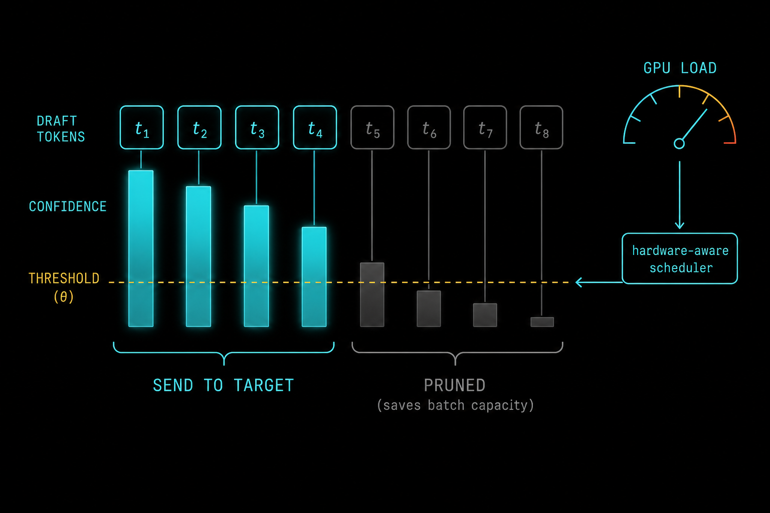
Step 6 — Fix Three: The Hardware-Aware Prefix Scheduler

A static confidence threshold is still a fixed policy, and fixed policies leave money on the table. The final DSpark component makes the verification decision jointly across all active requests, using the actual measured behaviour of the serving engine.

The scheduler works with two inputs. First, per-request survival curves from the calibrated confidence head. Second, a profiled SPS curve (steps per second as a function of total verification batch size) that captures how this specific engine on this specific hardware slows down as you stuff more tokens into a verification pass. The objective is to choose a verification prefix length for every request such that the expected system-wide token throughput (expected accepted tokens per step, multiplied by steps per second at the chosen batch size) is maximised. The algorithm greedily extends the prefixes with the highest survival probabilities, globally sorted across requests, and stops when adding more tokens would cost more in engine slowdown than it returns in expected accepted tokens.

# Hardware-aware prefix scheduling, conceptually
# For each active request r: survival curve a[r][j] = c1 * c2 * ... * cj
# Profiled: SPS(B) = engine steps/second at verification batch size B

candidates = all (request, position) extensions,
             sorted by survival probability, descending

B = R                       # every request verifies at least 1 token
best = expected_tokens(B) * SPS(B)

for (r, j) in candidates:
    B += 1                  # tentatively verify one more token for r
    throughput = expected_tokens(B) * SPS(B)
    if throughput > best:
        best = throughput
        extend request r to length j
    # low-survival tokens never justify their batch slot: pruned

The emergent behaviour is a self-regulating serving engine. Under light load, spare capacity means SPS barely drops as B grows, so the scheduler hands out long verification budgets (the paper reports roughly 4 to 6 tokens per request, versus the old MTP-1 baseline’s static 2) and individual users get their answers dramatically faster. Under heavy load, the SPS penalty bites, budgets shrink smoothly, and low-confidence tokens are pruned before they consume batch capacity that paying users need. Nobody tuned a knob; the optimum falls out of the profiled curve and the calibrated probabilities. It is the same design instinct behind congestion control in TCP: measure the system you actually have, not the system you wish you had.

Step 7 — The Results, Read Honestly

DeepSeek deployed DSpark (maximum draft length 5) inside the production serving engines of DeepSeek-V4-Flash and V4-Pro, under live user traffic, against the previous production baseline MTP-1. Headline results, straight from the paper:

• Per-user speed: 60–85% faster generation on V4-Flash, and 57–78% on V4-Pro, at matched aggregate throughput.
• Moderate service-level agreements: at an 80 tokens/second/user SLA on V4-Flash, aggregate throughput improved 51%; at 35 tok/s/user on V4-Pro, 52%.
• Strict SLAs: at 120 tok/s/user (Flash) the nominal advantage is 661% higher aggregate throughput, and at 50 tok/s/user (Pro) it is 406%.

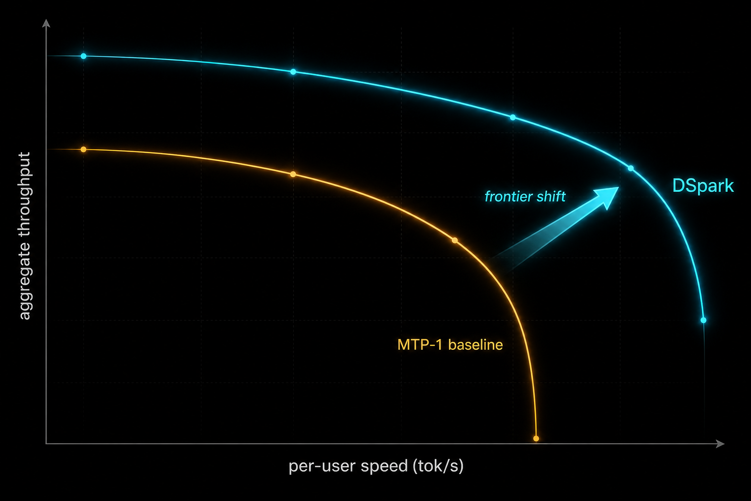
“Compared to the established production baseline (MTP-1), DSpark accelerates per-user generation speeds by 60%–85% at matched throughput levels. More importantly, by preventing severe throughput degradation under strict interactivity constraints, it enables performance tiers that were previously unattainable, shifting the Pareto frontier of our serving system.” — DeepSeek-AI, DSpark paper, Abstract

Now the honest reading of that 661% figure, because the paper itself insists on it and most summaries do not. At the strict 120 tok/s/user SLA, the old MTP-1 baseline is essentially falling off a cliff: it can only sustain a tiny concurrent batch while guaranteeing that speed, so the denominator of the comparison is nearly degenerate. The authors explicitly say they interpret the high-SLA points “primarily as evidence that DSpark extends the feasible interactivity frontier, rather than as a representative multiplicative speedup over a well-utilized baseline”. In plain terms: do not tell your boss DSpark makes serving seven times faster. Tell them it makes each user 60–85% faster at the same fleet capacity, and it keeps ultra-fast interactivity tiers commercially viable where the old system collapsed. That second claim is arguably more valuable, and it is the accurate one.

And because rejection sampling preserves the target distribution exactly (Step 2), all of these gains come at literally zero quality cost. This is not a quantisation trade-off or a distillation approximation. The output distribution is the target model’s, token for token.

Step 8 — Run It Yourself: The DeepSpec Repository

DeepSeek open-sourced the whole training and evaluation stack under the MIT licence as DeepSpec, alongside trained DSpark checkpoints.

“DeepSpec is a full-stack codebase for training and evaluating draft models for speculative decoding. It contains data preparation utilities, draft model implementations, training code, and evaluation scripts.” — DeepSpec README, deepseek-ai on GitHub

The repo implements three draft algorithms (Eagle3, DFlash, and DSpark) behind one training framework, so you can reproduce the paper’s comparisons like for like. The workflow is three stages, each feeding the next:

# 1. Install dependencies
python -m pip install -r requirements.txt

# 2. Data preparation: download prompts, regenerate target answers,
#    build the target cache.
#    WARNING from the README: the target cache can be very large,
#    roughly 38 TB for the default Qwen/Qwen3-4B setting.
#    See scripts/data/README.md before you fill a disk.

# 3. Train a draft model (default: single node, 8 GPUs)
bash scripts/train/train.sh
#    Select the algorithm via config_path, e.g.
#    config/dspark/dspark_qwen3_4b.py
#    Checkpoints land in ~/checkpoints/<project>/<exp>/step_*

# 4. Evaluate acceptance on benchmarks (gsm8k, math500, aime25,
#    humaneval, mbpp, livecodebench, mt-bench, alpaca, arena-hard-v2)
bash scripts/eval/eval.sh

If you do not want to train anything, released checkpoints exist for Qwen3-4B, Qwen3-8B, Qwen3-14B and Gemma-4-12B targets, for all three algorithms (for example deepseek-ai/dspark_qwen3_4b_block7 on Hugging Face). And DSpark is already wired into DeepSeek’s own flagship: the DeepSeek-V4-Pro-DSpark release is, per its model card, “not a new model. It is the same checkpoint with an additional speculative decoding module attached”. Same weights, same quality, faster serving.

Two practical notes from the README worth respecting. First, the released checkpoints were trained on target outputs in non-thinking mode; if your target runs in thinking mode or a narrow domain, fine-tune the draft model again or your acceptance rates will disappoint. Second, if you benchmark against these checkpoints in your own work, align your setup with the repo’s training settings, otherwise the comparison is meaningless. Reproducibility discipline, stated plainly in the README, and rarer than it should be.

When the Old Ways Are Actually Fine

Balance, because credibility demands it. DSpark solves a high-concurrency production serving problem. Not every deployment has one.

• Single-user or low-concurrency inference. If you are running a local model for yourself, batch capacity contention does not exist. A plain parallel or autoregressive drafter, or even vanilla decoding on a small model, may be all you need. The confidence head and scheduler add engineering surface you will not exercise.
• Offline batch workloads. If nobody is waiting on per-token latency (overnight evaluation runs, dataset generation), per-user interactivity is irrelevant. Maximise raw throughput with big batches and skip speculation entirely; decode is less memory-starved when batches are already large.
• Heavily structured domains with an autoregressive drafter that already works. On code-only workloads, acceptance rates are naturally high (the paper measured 67.6% baseline acceptance on code versus 45.7% on chat), so the marginal gain from confidence scheduling is smaller. If Eagle3 is already deployed and hitting your latency targets, migrating has a real cost.
• Tiny models. If the target model is small enough that a forward pass is fast anyway, the drafter overhead can eat the gains. Speculative decoding pays off when the target is expensive relative to the draft.

The pattern generalising all four: DSpark’s genius is load-aware resource allocation under contention. No contention, less genius required.

What to Check Right Now

• Find out whether your serving stack uses speculative decoding at all — vLLM, SGLang and TensorRT-LLM all support drafter-based speculation; if you serve LLMs at any scale and this is switched off, you are leaving 2x-class latency gains unclaimed.
• Measure your acceptance rate by domain — log accepted length per verification cycle, split by workload type. If chat traffic shows sub-50% acceptance while code shows 70%+, you are exactly the profile that fixed-length verification punishes, and confidence-style gating will help.
• Profile your engine’s throughput-versus-batch curve — DSpark’s scheduler depends on knowing SPS(B) for the actual hardware. Even without adopting DSpark, this profile tells you where your serving sweet spot is. Most teams have never measured it.
• Check your drafter’s block length against its acceptance decay — if you use a parallel drafter, plot per-position acceptance. Sharp suffix decay means you are drafting tokens that never survive; either shorten the block or adopt a semi-autoregressive head.
• Clone DeepSpec and run the evaluation on a released checkpoint — the eval path needs no 38 TB cache, just a target model and a downloaded draft checkpoint. An afternoon of work gets you first-hand acceptance numbers on your own prompts.
• Re-read the strict-SLA claims in any coverage you consume — if a summary quotes “700% faster” without mentioning that the baseline was degenerate at that operating point, treat the rest of the summary with matching suspicion. The paper’s own framing is the frontier shift, not the multiplier.

Video Attribution

This guide was prompted by AI Search’s video walkthrough of the DSpark release, which is a good gateway into the topic; the technical details above were verified against and expanded from the primary sources: the DSpark paper, the DeepSpec repository, and the DeepSeek-V4-Pro-DSpark model card.

nJoy 😉