Trade Management with ATR

ATR-Based Trade Management
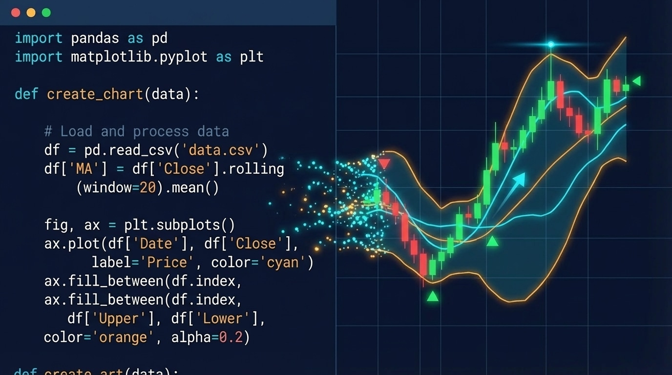
ATR-based stop-loss and take-profit levels adapt to market volatility

Ichimoku Trading Series: Part 6 of 10 | ← Previous | View Full Series

ATR-Based Risk Management

Instead of fixed pip distances, we use the Average True Range (ATR) to adapt our stops to current market volatility.

Why ATR?

  • In volatile markets → wider stops (avoid noise)
  • In calm markets → tighter stops (maximise R:R)
  • Automatically adapts to the instrument

The Formulas

Stop-Loss Distance

SL_distance = ATR × ATR_MULT_SL

# For long: SL = entry - SL_distance
# For short: SL = entry + SL_distance

Take-Profit Distance

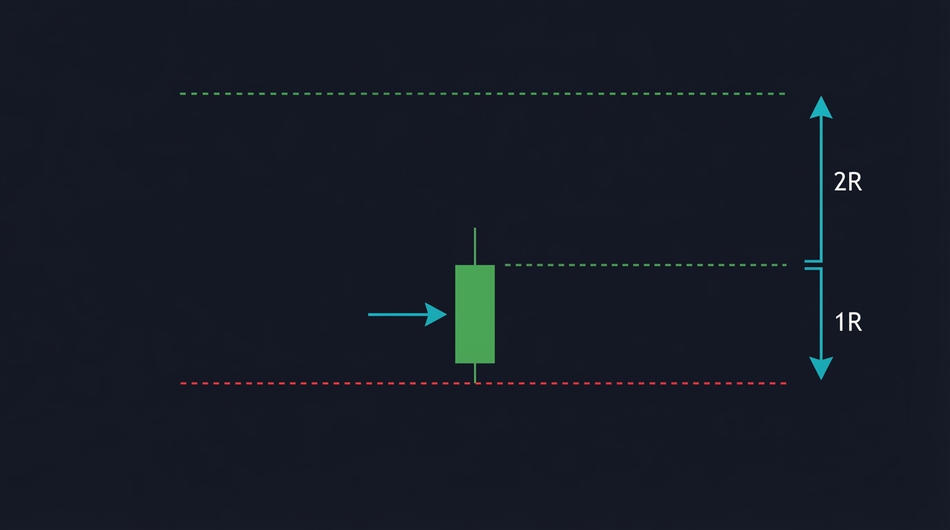
TP_distance = SL_distance × RR_MULT_TP

# For long: TP = entry + TP_distance
# For short: TP = entry - TP_distance

Default Parameters

ATR_LEN      = 14      # ATR lookback period
ATR_MULT_SL  = 2.0     # SL = ATR × 2
ATR_MULT_TP  = 4.0     # TP = ATR × 4  (gives 2R)

With these defaults:

  • Risk-Reward Ratio = 4 / 2 = 2R
  • Win only 33% of the time to break even
  • Our 53-69% win rate means consistent profits

Optimisation Insights

From backtesting results:

ATR Multiplier Best RR Ratio Returns
1.0 (tight) 2.5-2.9 Highest
1.5 (medium) 1.5-2.0 Good
2.0 (wide) 1.0-1.5 Moderate

Key Finding: Tight stops with high R:R work best!

“The best set of parameters is decreasing like this. Either you have a high stop-loss distance and a low risk-reward ratio, or you have a low ATR multiplier or stop-loss distance and a high risk-reward ratio — which actually is working the best for this strategy.”

Why Tight Stops Work Here

Because we are entering at cloud bounces (retracements):

“We are squeezing our entry position to the retracement to the minimum of the retracement when we are dipping within inside of the cloud and just getting out of it. So this is why you do not need a very wide stop-loss distance.”

Code Implementation

# Risk settings
ATR_LEN      = 14
ATR_MULT_SL  = 1.5     # Tight stop-loss
ATR_MULT_TP  = 3.0     # Higher R:R (2R)

# In strategy:
sl_dist = atr * self.atr_mult_sl
tp_dist = sl_dist * self.rr_mult_tp

if signal == 1:  # Long entry
    sl = close - sl_dist
    tp = close + tp_dist
    self.buy(size=0.99, sl=sl, tp=tp)

elif signal == -1:  # Short entry
    sl = close + sl_dist
    tp = close - tp_dist
    self.sell(size=0.99, sl=sl, tp=tp)
Coming Up Next: Our rules are defined — let us build the Python backtesting infrastructure to test them. Continue to Part 7 →

Results Analysis and Next Steps

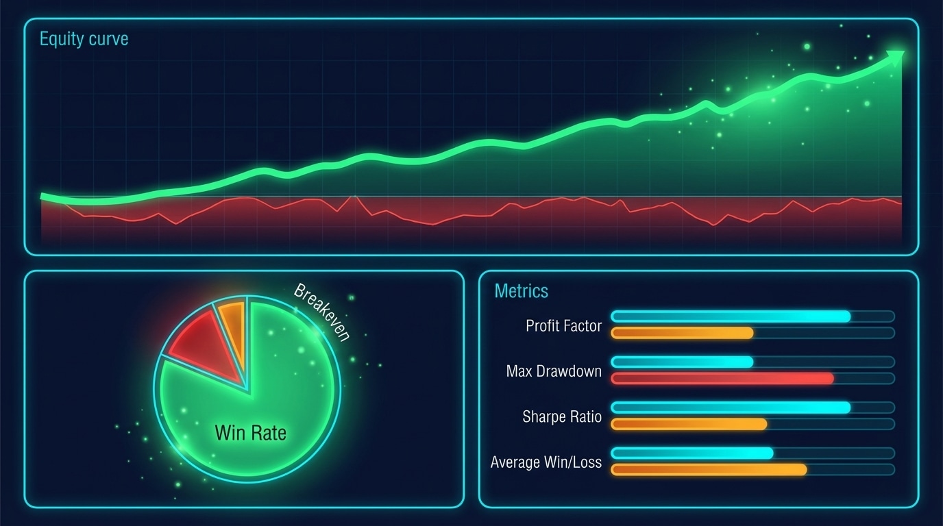
Trading Results Dashboard
Final backtest results showing consistent profitability across multiple metrics

Ichimoku Trading Series: Part 10 of 10 (Final) | ← Previous | View Full Series

Final Backtest Results

Single Asset (USDCHF) – Optimised Parameters

Metric Value
Annual Return 43%
Buy & Hold -5.7%
Win Rate 69%
Max Drawdown -21% (with leverage)
Sharpe Ratio 1.38
Trades 13

Without Leverage

Metric Value
Annual Return ~4%
Max Drawdown -2%
Sharpe Ratio Higher

Multi-Asset Summary

Symbol Return [%] MaxDD [%] Win Rate [%] Trades
EURUSD=X 28.5 -6.3 53.8 15
USDJPY=X 35.2 -8.1 61.5 13
GBPUSD=X 22.1 -7.2 50.0 14
USDCHF=X 43.0 -6.0 69.2 13
AVERAGE 32.2 -6.9 58.6 14

Key Insights

1. The Strategy is SELECTIVE

“Only one issue is that we have only 13 trades in here and that is the main weak point of this strategy. It is very selective.”

This is actually a feature:

  • Fewer trades = lower commission costs
  • Each trade has high conviction
  • Manageable for manual oversight

2. Better for Trending Markets

“I do not think Forex is the best place to test this strategy… It works better on stocks, especially winning stocks.”

The strategy excels when:

  • Markets have clear trends
  • Retracements to cloud are clean
  • Less choppy price action

3. Best as a Signal Generator

“Ideally, we would deploy this strategy online live, but it will not trade on its own. It will actually send you signals… emails or notifications whenever the pattern is there and then you can jump in.”

The 4-hour timeframe means:

  • No rush to enter
  • Time to verify setup manually
  • Filter out borderline signals

Recommended Deployment

Option 1: Alert System

Strategy runs on server → Detects signal → Sends email/Telegram alert → You verify and enter manually

Option 2: Semi-Automated

Strategy generates signal → Places order with your manual approval → Manages SL/TP automatically

Ideas for Improvement

1. Filter Long Candles

“It would be good to add one additional filter where if candles are way too long, we are going to discard the signal because we want to squeeze the best risk-reward ratio.”

# Reject signals where entry candle is too large
max_candle_atr = 1.5
candle_range = abs(df["Close"] - df["Open"])
valid_entry = candle_range < (df["ATR"] * max_candle_atr)

2. Add Volume Confirmation

Higher volume on the bounce confirms institutional interest.

3. Multiple Timeframe Analysis

Use daily chart for trend, 4H for entry.

4. Asset-Specific Optimisation

Each instrument has different optimal parameters.

Final Thoughts

This Ichimoku + EMA strategy provides:

  • ✔ Clear, mechanical rules
  • ✔ Trend-following with retracement entries
  • ✔ Proper risk management
  • ✔ Realistic backtesting (no look-ahead bias)

The 28-43% returns with controlled drawdowns make this a solid addition to any trader toolkit.

Download & Experiment

Full Code: GitHub – Ichimoku_Trend

“You can download the code, tweak the parameters, and test the strategy on different assets.”

🎉 Congratulations! You have completed the Ichimoku Cloud Trading Strategy course. Return to Series Index

Understanding the Kumo Cloud

Understanding the Kumo Cloud
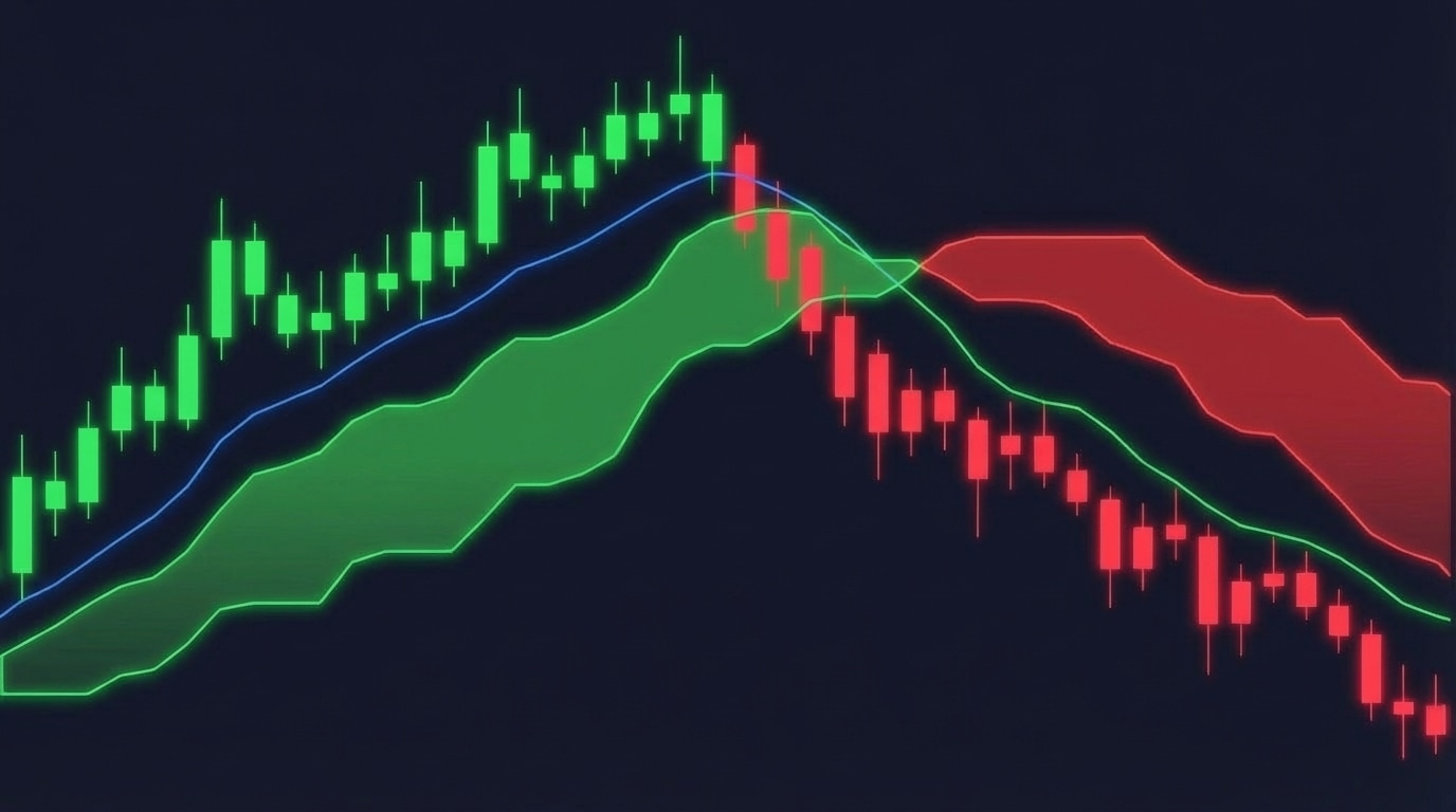
Bullish and bearish cloud formations with price piercing through

Ichimoku Trading Series: Part 3 of 10 | ← Previous | View Full Series

The Cloud (Kumo)

The space between Senkou Span A and Senkou Span B creates the “cloud” — a dynamic zone of support and resistance.

Bullish Cloud (Green)

When Span A > Span B, the cloud is bullish:

Price → [Span A (top)] → [Span B (bottom)]

Bearish Cloud (Red)

When Span B > Span A, the cloud is bearish:

Price → [Span B (top)] → [Span A (bottom)]

What the Cloud Tells Us

1. Trend Direction

  • Price above cloud = Bullish trend
  • Price below cloud = Bearish trend
  • Price inside cloud = Consolidation/uncertainty

2. Support/Resistance Strength

  • Thick cloud = Strong support/resistance
  • Thin cloud = Weak support/resistance, easier breakouts

3. Future Sentiment

The cloud projects forward, showing where support/resistance WILL BE.

Critical: Avoiding Look-Ahead Bias

The Problem

Standard Ichimoku implementations shift Span A and Span B 26 periods into the future. In backtesting, this means your strategy “knows” future support/resistance levels — data leakage!

Our Solution

# We use UNshifted spans for signal logic
span_a_raw = (tenkan_line + kijun_line) / 2.0  # raw (no forward shift)
span_b_raw = (h.rolling(senkou_b).max() + l.rolling(senkou_b).min()) / 2.0  # raw

From the source material:

“I decided to compute the Ichimoku manually for one reason… The Ichimoku by default shifts or reads a bit in the future. This would be a look-ahead bias for our backtesting.”

Cloud Boundaries for Signals

cloud_top = df[["ich_spanA", "ich_spanB"]].max(axis=1)
cloud_bot = df[["ich_spanA", "ich_spanB"]].min(axis=1)

Cloud Twist

When the cloud changes colour (Span A and Span B cross), it signals a potential trend reversal. This is called a Kumo Twist or Senkou Span Cross.

  • Bullish Twist: Span A crosses above Span B → Cloud turns green
  • Bearish Twist: Span A crosses below Span B → Cloud turns red

Coming Up Next: The cloud tells us about support and resistance, but we need a trend filter to avoid false signals. In Part 4, we add our EMA Trend Filter. Continue to Part 4 →

Parameter Optimization

Parameter Optimisation Heat Map
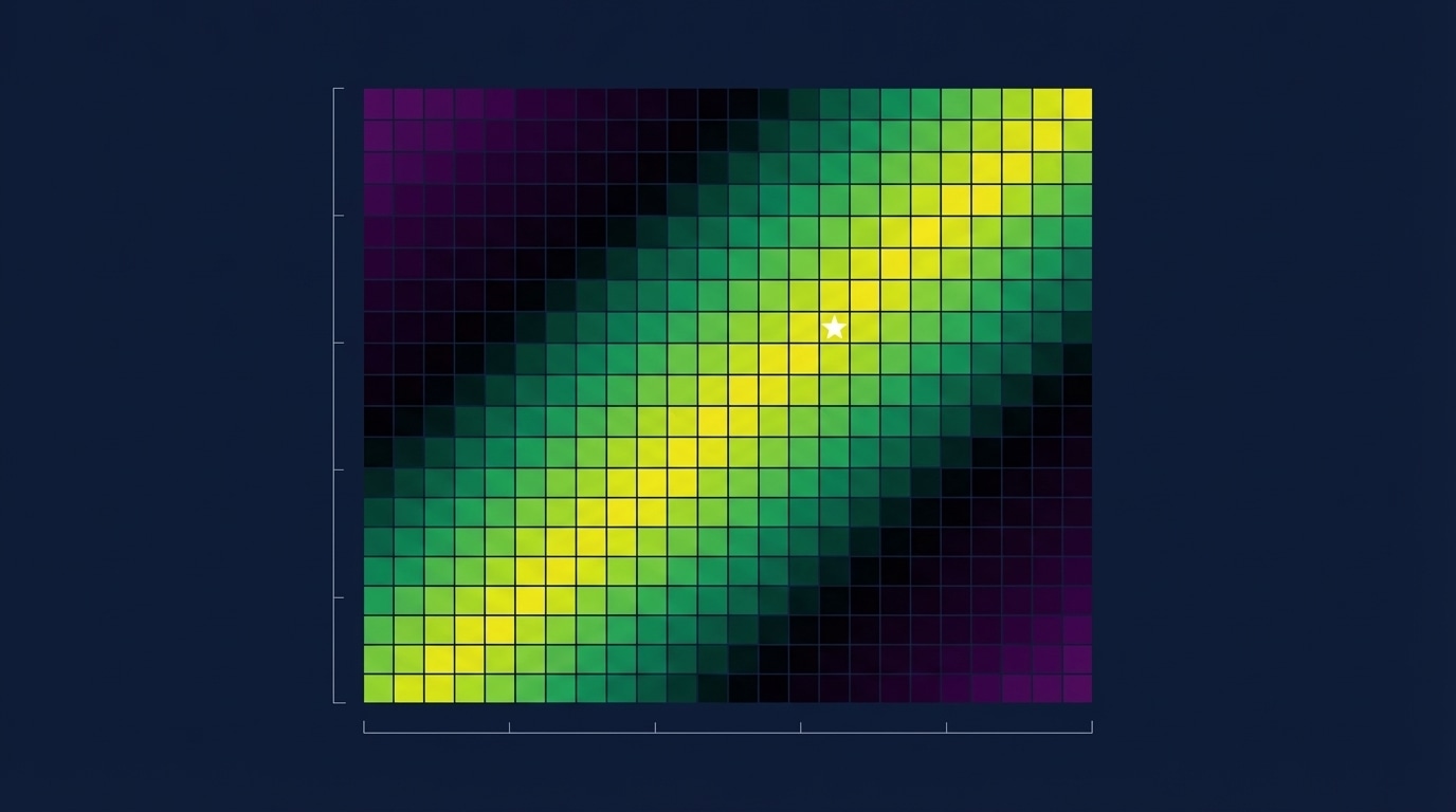
Heat map visualisation showing optimal parameter combinations

Ichimoku Trading Series: Part 9 of 10 | ← Previous | View Full Series

The Optimisation Challenge

We have two key parameters to tune:

  1. ATR Multiplier (stop-loss distance)
  2. Risk-Reward Multiplier (take-profit distance)

Grid Search Approach

# Parameter ranges
atr_range = np.arange(1.0, 2.5, 0.1)  # 1.0 to 2.4
rr_range  = np.arange(1.0, 3.0, 0.1)  # 1.0 to 2.9

# Run optimization
stats, heatmap = bt.optimize(
    atr_mult_sl=atr_range,
    rr_mult_tp=rr_range,
    maximize="Return [%]",
    constraint=lambda param: param.rr_mult_tp >= 1,
    return_heatmap=True
)

Multi-Asset Testing

Test across multiple instruments to ensure robustness:

SYMBOLS = [
    "EURUSD=X", "USDJPY=X", "GBPUSD=X", 
    "AUDUSD=X", "USDCHF=X", "USDCAD=X", "NZDUSD=X"
]

def run_all_assets(symbols, start, end, interval, cash, commission):
    rows = []
    for sym in symbols:
        try:
            stats, _, _ = run_backtest(
                symbol=sym, start=start, end=end, 
                interval=interval, cash=cash, commission=commission,
                show_plot=False
            )
            rows.append({
                "Symbol": sym,
                "Return [%]": stats.get("Return [%]"),
                "MaxDD [%]": stats.get("Max. Drawdown [%]"),
                "Win Rate [%]": stats.get("Win Rate [%]"),
                "Trades": stats.get("# Trades"),
            })
        except Exception as e:
            print(f"Warning {sym}: {e}")
    
    return pd.DataFrame(rows)

summary = run_all_assets(SYMBOLS, START, END, INTERVAL, CASH, COMMISSION)
print(summary)

Understanding the Heat Map

The optimisation produces a heat map showing returns for each parameter combination.

Key Pattern: The Diagonal

“Notice those ridges, those clusters of returns… It is showing this decreasing slope. And this is totally normal.”

Why the diagonal?

  • High ATR multiplier = wider stop-loss → needs lower R:R
  • Low ATR multiplier = tighter stop-loss → can use higher R:R

“Either you have a high stop-loss distance and a low risk-reward ratio, OR you have a low ATR multiplier and a high risk-reward ratio — which actually is working the best for this strategy.”

Optimal Zone

ATR Mult RR Mult Expected Return
1.0-1.3 2.5-2.9 35-43%
1.4-1.7 1.8-2.2 25-35%
1.8-2.4 1.0-1.5 15-25%

Heat Map Visualisation Code

import plotly.express as px

def plot_heatmap(heat, metric_name="Return [%]", min_return=10):
    """Plot optimization heatmap with threshold filtering."""
    
    # Pivot to matrix form
    zdf = heat.pivot(index="atr_mult_sl", columns="rr_mult_tp", values=metric_name)
    
    # Create heatmap
    fig = px.imshow(
        zdf.values,
        x=zdf.columns,
        y=zdf.index,
        color_continuous_scale="Viridis",
        labels=dict(x="RR Multiplier", y="ATR Multiplier", color=metric_name),
        title=f"Optimization Heatmap - {metric_name}"
    )
    
    return fig

Avoiding Overfitting

  • Test on multiple assets, not just one
  • Use walk-forward analysis
  • Look for robust parameter zones, not single optimal points
  • Consider the diagonal pattern — many combinations work

Coming Up Next: Optimisation complete — let us analyse what we found and draw conclusions in our final part. Continue to Part 10 →

Building the Strategy Class

Strategy Class Architecture
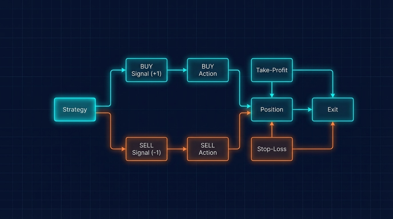
The Strategy class handles signal processing and position management

Ichimoku Trading Series: Part 8 of 10 | ← Previous | View Full Series

The backtesting.py Framework

The backtesting library uses a class-based approach where:

  • init() runs once at the start
  • next() runs on every candle

Complete Strategy Class

from backtesting import Strategy

class SignalStrategy(Strategy):
    """
    Ichimoku + EMA trend-following strategy.
    
    Entry: Pre-computed signal column (+1 long, -1 short)
    Exit: ATR-based SL and RR-based TP
    """
    
    # Class-level parameters (can be optimized)
    atr_mult_sl: float = 1.5   # SL distance = ATR x this
    rr_mult_tp:  float = 2.0   # TP distance = SL x this
    
    def init(self):
        """Initialize indicators (we pre-compute, so nothing needed here)."""
        pass
    
    def next(self):
        """Called on every bar. Check for signals and manage positions."""
        i = -1  # Current bar
        signal = int(self.data.signal[i])   # +1 long, -1 short, 0 none
        close  = float(self.data.Close[i])
        atr    = float(self.data.ATR[i])
        
        # Safety check
        if not (atr > 0):
            return
        
        # --- Manage open trades ---
        if self.position:
            # Let SL/TP handle exits automatically
            return
        
        # --- New entry logic ---
        sl_dist = atr * self.atr_mult_sl
        tp_dist = sl_dist * self.rr_mult_tp
        
        if signal == 1:  # LONG entry
            sl = close - sl_dist
            tp = close + tp_dist
            self.buy(size=0.99, sl=sl, tp=tp)
        
        elif signal == -1:  # SHORT entry
            sl = close + sl_dist
            tp = close - tp_dist
            self.sell(size=0.99, sl=sl, tp=tp)
Key Design Decisions

1. Pre-Computed Signals

We calculate signals BEFORE backtesting (in pandas), then the strategy just reads them. This is cleaner and faster.

2. Position Check

if self.position:
    return

We do not stack trades — one position at a time.

3. Size = 0.99

self.buy(size=0.99, sl=sl, tp=tp)

Using 99% of available equity leaves room for rounding.

Running the Backtest

def run_backtest(symbol, start, end, interval, cash, commission, show_plot=True):
    # Prepare data
    df = fetch_data(symbol, start, end, interval)
    df = add_ichimoku(df)
    df["EMA"] = ta.ema(df.Close, length=100)
    df = MovingAverageSignal(df, back_candles=7)
    df = createSignals(df, lookback_window=10, min_confirm=7)
    df = df.dropna()
    
    # Create backtest
    bt = Backtest(
        df,
        SignalStrategy,
        cash=cash,
        commission=commission,
        trade_on_close=True,
        exclusive_orders=True,
        margin=1/10,  # 10x leverage
    )
    
    # Run and display results
    stats = bt.run()
    print(f"n=== {symbol} Signal Strategy ===")
    print(stats)
    
    if show_plot:
        bt.plot(open_browser=False)
    
    return stats, df, bt

# Execute
stats, df, bt = run_backtest(
    symbol="USDCHF=X",
    start="2023-10-01",
    end="2024-10-01", 
    interval="4h",
    cash=1_000_000,
    commission=0.0002
)

Example Output

=== USDCHF=X Signal Strategy ===
Return [%]                     28.5
Sharpe Ratio                    1.02
Max. Drawdown [%]              -6.3
Avg. Drawdown [%]              -3.7
Win Rate [%]                   53.8
# Trades                         13
Exposure Time [%]              42.1

Coming Up Next: Our strategy is coded — now let us optimise parameters using grid search and visualise results with heat maps. Continue to Part 9 →

Python Backtesting Setup

Python Backtesting Setup
Setting up the Python environment for algorithmic trading backtests

Ichimoku Trading Series: Part 7 of 10 | ← Previous | View Full Series

Required Libraries

from __future__ import annotations
import warnings
warnings.filterwarnings("ignore", category=FutureWarning)

import numpy as np
import pandas as pd
import pandas_ta as ta        # Technical analysis
import yfinance as yf         # Free market data
from backtesting import Backtest, Strategy

Installation

pip install numpy pandas pandas-ta yfinance backtesting plotly

Fetching Market Data

def fetch_data(symbol: str, start: str, end: str, interval: str) -> pd.DataFrame:
    """
    Fetch OHLCV data from Yahoo Finance.
    
    Parameters:
    - symbol: "EURUSD=X", "AAPL", "BTC-USD", etc.
    - start/end: "2023-01-01" format
    - interval: "1h", "4h", "1d"
    """
    df = yf.download(symbol, start=start, end=end, interval=interval,
                     auto_adjust=True, progress=False, threads=False)
    
    if df.empty:
        raise ValueError(f"No data returned for {symbol}")
    
    # Handle MultiIndex columns (newer yfinance versions)
    if isinstance(df.columns, pd.MultiIndex):
        df = df.xs(symbol, axis=1, level=1)
    
    # Standardize column names
    df.columns = [c.title() for c in df.columns]
    return df.dropna()

Adding Ichimoku Indicators

def add_ichimoku(df: pd.DataFrame,
                 tenkan: int = 9,
                 kijun: int = 26,
                 senkou_b: int = 52) -> pd.DataFrame:
    """
    Build bias-safe Ichimoku columns for SIGNAL logic.
    - Raw spans (no forward shift) to avoid look-ahead bias
    """
    out = df.copy()
    h, l, c = out["High"], out["Low"], out["Close"]
    
    # Compute lines manually (bias-free)
    tenkan_series = (h.rolling(tenkan).max() + l.rolling(tenkan).min()) / 2.0
    kijun_series  = (h.rolling(kijun).max() + l.rolling(kijun).min()) / 2.0
    
    # Raw spans (NO forward shift!)
    span_a_raw = (tenkan_series + kijun_series) / 2.0
    span_b_raw = (h.rolling(senkou_b).max() + l.rolling(senkou_b).min()) / 2.0
    
    out["ich_tenkan"] = tenkan_series
    out["ich_kijun"]  = kijun_series
    out["ich_spanA"]  = span_a_raw
    out["ich_spanB"]  = span_b_raw
    
    # Add ATR for trade management
    out["ATR"] = ta.atr(out["High"], out["Low"], out["Close"], length=14)
    
    # Add EMA for trend filter
    out["EMA"] = ta.ema(out["Close"], length=100)
    
    # Drop warmup NaNs
    return out.dropna()

Putting It Together

# Configuration
SYMBOL   = "EURUSD=X"
START    = "2023-10-01"
END      = "2024-10-01"
INTERVAL = "4h"
CASH     = 100_000
COMMISSION = 0.0002  # 0.02%

# Fetch and prepare data
df = fetch_data(SYMBOL, START, END, INTERVAL)
df = add_ichimoku(df)
df = MovingAverageSignal(df, back_candles=7)
df = createSignals(df, lookback_window=10, min_confirm=7)
df = df.dropna()

print(f"Data shape: {df.shape}")
print(df.tail())

Data Verification

Your DataFrame should now have these columns:

Open, High, Low, Close, Volume,
ich_tenkan, ich_kijun, ich_spanA, ich_spanB,
ATR, EMA, EMA_signal, signal

Coming Up Next: With data flowing, let us build our Strategy class that the backtester will execute. Continue to Part 8 →

Introduction to Ichimoku Cloud Trading

Ichimoku Cloud Trading Strategy Overview
The Ichimoku Cloud combined with EMA trend filtering creates high-probability trade setups

Ichimoku Trading Series: Part 1 of 10 | View Full Series

What You Will Build

In this 10-part series, you will learn to automate a trading strategy that combines:

  • Ichimoku Cloud (Ichimoku Kinko Hyo) for entry signals
  • EMA 100 as a trend filter
  • ATR-based stop-loss and take-profit management

The strategy achieved ~40% yearly returns in backtests across multiple FX pairs on the 4-hour timeframe, with a 53-69% win rate and controlled drawdowns.

Why This Strategy Works

The core principle is simple but powerful:

  1. Trade WITH the trend — The EMA filter ensures we only take trades in the prevailing market direction
  2. Wait for retracements — The Ichimoku Cloud identifies perfect pullback entries
  3. Enter at the bounce — When price dips INTO the cloud and closes OUTSIDE, the retracement is likely over

Visual Signal Example

Green triangles = Long signals (buy)
Red triangles = Short signals (sell)

The strategy only takes trades that align with both the EMA trend AND the Ichimoku setup.

What Makes This Approach Unique

Problem with Standard Ichimoku

Most Ichimoku implementations suffer from look-ahead bias — they shift the cloud forward in time, which gives misleadingly good backtest results.

Our Solution

We compute the Ichimoku components without forward-shifting the spans, ensuring honest backtesting results that translate to real trading.

Key Backtest Results

Metric Value
Annual Return 28-43%
Win Rate 53-69%
Max Drawdown -6% to -21%
Sharpe Ratio 1.0-1.38
Trades per Year ~13 (selective)

Important Note: The strategy is SELECTIVE — only ~13 trades per year. This is a feature, not a bug. Quality over quantity.

Course Overview

Over the next 10 parts, you will learn:

  • Part 2: The Five Ichimoku Components
  • Part 3: Understanding the Kumo Cloud
  • Part 4: EMA Trend Filter
  • Part 5: Entry Signal Conditions
  • Part 6: Trade Management with ATR
  • Part 7: Python Backtesting Setup
  • Part 8: Building the Strategy Class
  • Part 9: Parameter Optimisation
  • Part 10: Results Analysis & Next Steps

Prerequisites

  • Basic Python knowledge
  • Understanding of candlestick charts
  • Familiarity with trading concepts (SL, TP, R:R)

Coming Up Next: In Part 2, we will dive deep into the five Ichimoku components and understand exactly what each line tells us about market structure. Continue to Part 2 →

Concept Vectors and Analogy in LLMs

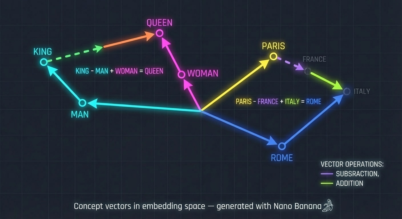
LLM Architecture Series – Bonus Lesson. In earlier lessons you saw how tokens become vectors. This article goes deeper into what those vectors mean and how simple arithmetic on them can reveal structure in concepts.

Concept vectors in embedding space

Concept vectors in embedding space, generated with Nano Banana.

(more…)

The Complete LLM Pipeline – Putting It All Together

LLM Architecture Series – Lesson 20 of 20. We have visited every component of the architecture. This lesson ties them together into a single mental model.

By walking through a full end to end example you can see how tokenization, embeddings, attention, MLPs, and the output layer cooperate to produce text.

(more…)

Scaling LLMs – nano-GPT to GPT-3

LLM Architecture Series – Lesson 19 of 20. You now understand the core architecture. Scaling is about what happens when we make models wider, deeper, and train them on more data.

Surprisingly, performance often follows smooth scaling laws, which lets practitioners predict the benefit of using larger models.

(more…)