Fine-Tuning AI Models Explained

Fine-tuning

Fine-Tuning: Adapting Pre-trained Models

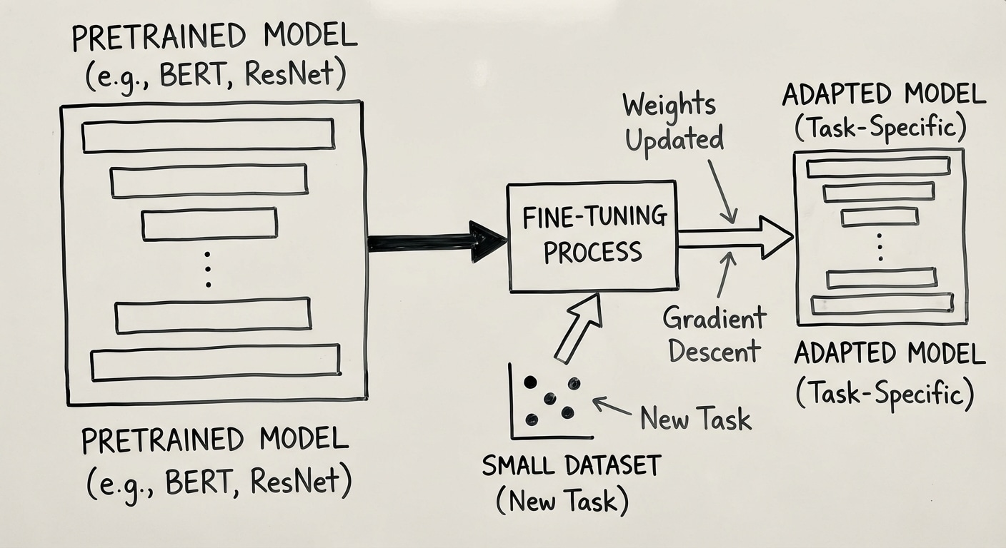
Fine-tuning transfers knowledge from large pre-trained models to specific tasks with limited data. This paradigm revolutionized AI by making powerful models accessible without requiring massive datasets or compute budgets for each new application.

The process involves taking a model pre-trained on massive general data, then continuing training on task-specific data with a lower learning rate. The pre-trained weights provide excellent initialisation, and fine-tuning adapts them to the new domain.

Different strategies trade off between performance and efficiency. Full fine-tuning updates all parameters for best results but requires significant compute. LoRA adds small trainable matrices alongside frozen weights, achieving 90%+ of full fine-tuning performance with a fraction of parameters.

Best practices include using lower learning rates than pre-training, employing warmup steps, monitoring validation loss for early stopping, and considering gradual unfreezing where deeper layers train first before unfreezing earlier layers.

GPT Architecture Explained

GPT

GPT: Inside Large Language Models

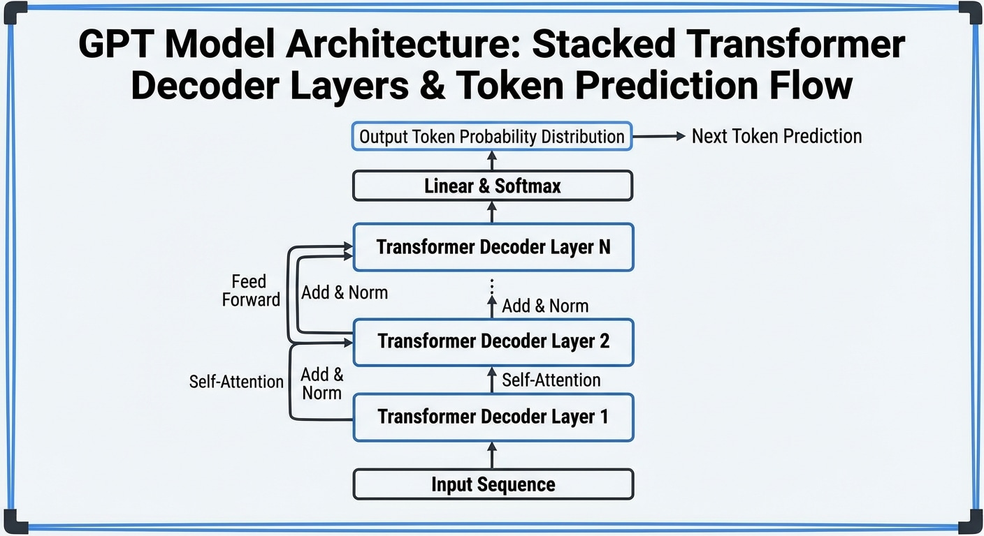
GPT (Generative Pre-trained Transformer) uses a decoder-only architecture to generate text token by token. Understanding its internals reveals how modern AI achieves remarkable language capabilities through elegant architectural choices.

Each token receives embedding plus positional encoding, then passes through stacked Transformer blocks. Each block contains masked self-attention (can only attend to previous tokens) and feed-forward networks. This autoregressive structure enables coherent text generation.

Scale proves critical for emergent capabilities. GPT-2 had 1.5B parameters, GPT-3 scaled to 175B, and GPT-4 reportedly exceeds a trillion. With scale comes surprising abilities: few-shot learning, reasoning, and code generation that emerge without explicit training.

Generation works by processing input tokens through all layers, predicting probability distribution over vocabulary for the next token, sampling from that distribution, appending the result, and repeating. Temperature and top-p sampling control creativity versus coherence.

Dropout Regularization Explained

Dropout

Dropout: Regularization Through Randomness

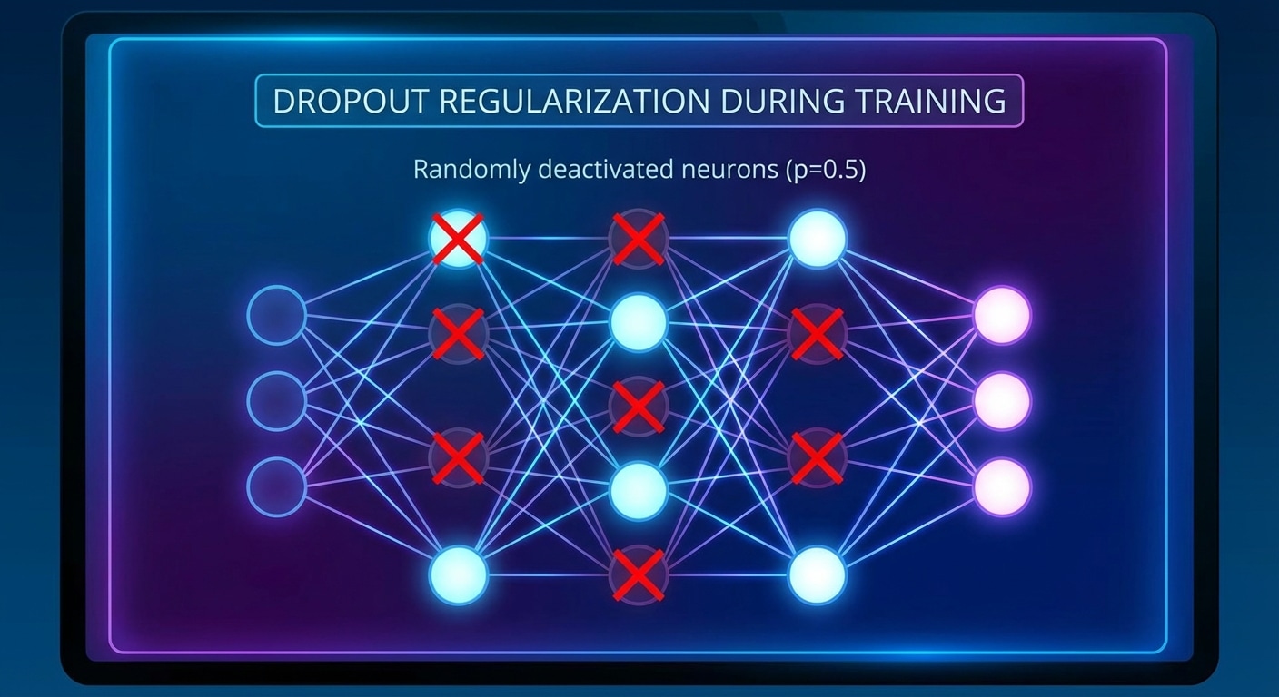
Dropout prevents overfitting by randomly deactivating neurons during training. This forces the network to learn redundant representations and prevents co-adaptation where neurons rely too heavily on specific other neurons being present.

During training, each neuron is kept with probability p, typically 0.5 for hidden layers and 0.8-0.9 for input layers. During inference, all neurons are active with weights scaled by p to maintain expected values. This creates an ensemble effect.

Dropout can be viewed as training many different subnetworks simultaneously, then averaging their predictions at test time. This ensemble interpretation explains its strong regularization effect without significant computational overhead.

While less common in modern architectures that use BatchNorm heavily, dropout remains valuable for fully connected layers and in specific contexts. Understanding when and where to apply it helps build robust models.

Batch Normalization Explained

BatchNorm

Batch Normalisation: Stabilizing Training

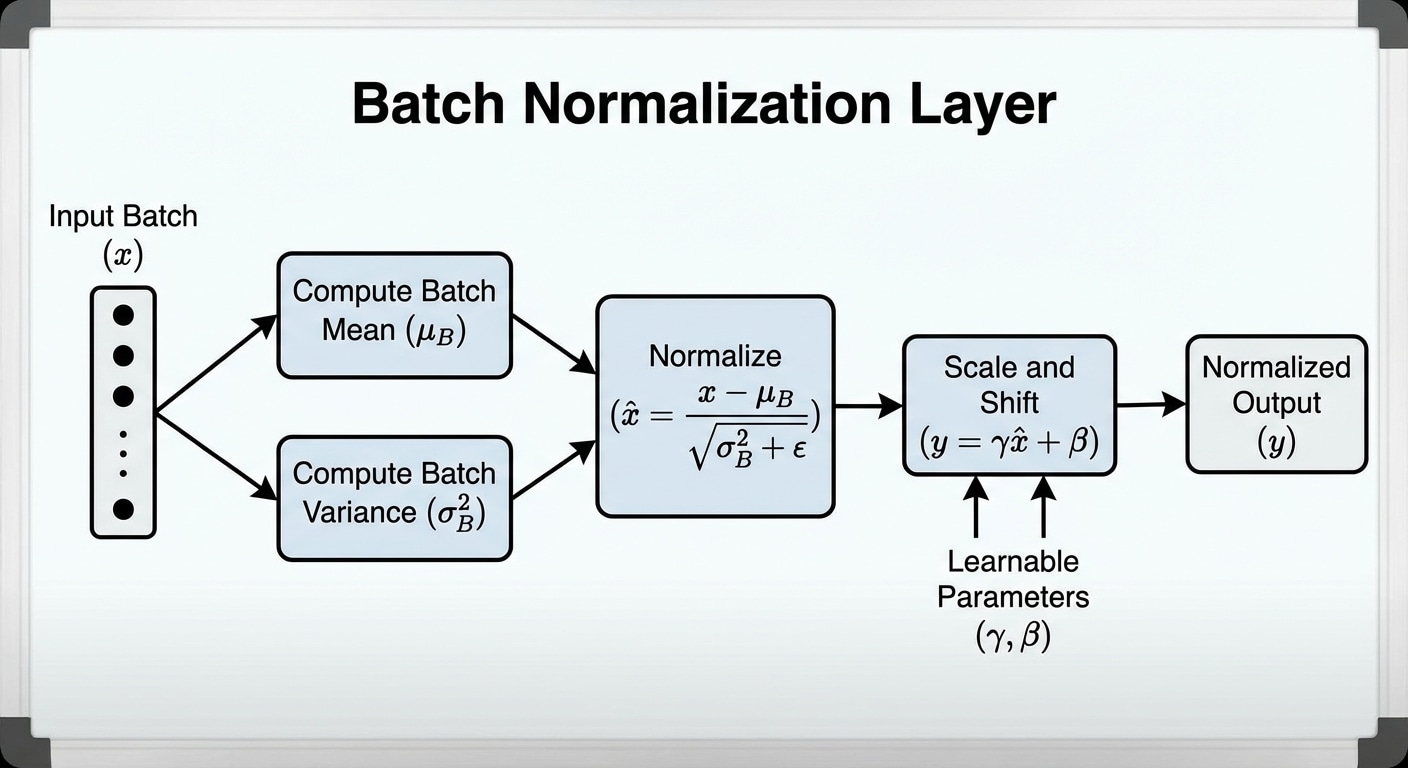
Batch normalisation dramatically improved training stability and speed when introduced in 2015. By normalising layer inputs, it reduces internal covariate shift and allows much higher learning rates, accelerating convergence significantly.

For each mini-batch, BatchNorm calculates mean and variance of activations, normalises them to zero mean and unit variance, then applies learnable scale and shift parameters. This standardisation stabilizes the distribution of inputs to each layer.

Benefits extend beyond training speed. BatchNorm acts as a regularizer due to noise from batch statistics, often reducing or eliminating the need for dropout. It also reduces sensitivity to weight initialisation, making networks easier to train.

Layer Normalisation offers an alternative for Transformers, normalising across features instead of batch dimension. This works with any batch size and is essential for sequence models where batch statistics can be noisy.

Overfitting vs Underfitting Explained

Overfitting

The Generalisation Challenge

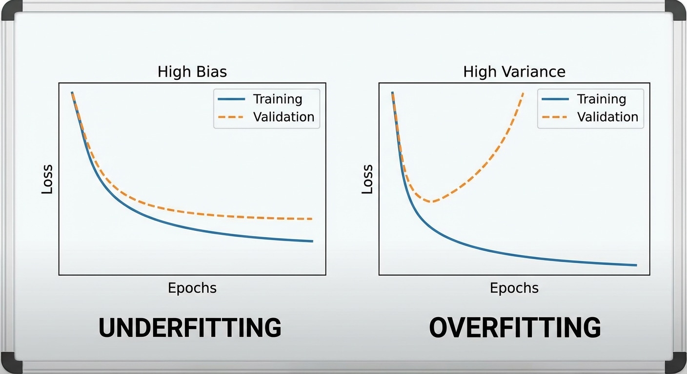
The core challenge in machine learning is generalising from training data to new examples. A model that memorises training data perfectly but fails on new data is useless. Understanding overfitting and underfitting is essential for building models that actually work in production.

Underfitting occurs when the model is too simple to capture patterns. High bias leads to poor performance on both training and test data. Solutions include increasing model capacity, adding features, training longer, or reducing regularization.

Overfitting happens when the model memorises training data including noise. High variance means great training performance but poor test performance. Solutions include more training data, regularization techniques, dropout, early stopping, and data augmentation.

The bias-variance tradeoff underlies this challenge. Simple models have high bias but low variance. Complex models have low bias but high variance. The goal is finding the sweet spot where total error is minimised for your specific application.

Gradient Descent Optimization Explained

Gradient Descent

Gradient Descent: Finding Optimal Solutions

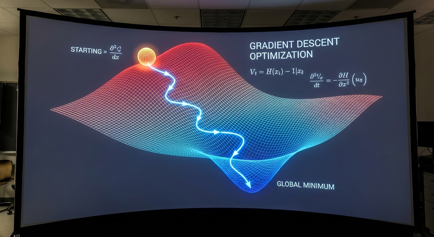
Gradient descent is the optimisation engine powering machine learning. It finds minimum error by iteratively moving in the direction of steepest descent on the loss surface. Understanding this algorithm is fundamental to training any neural network effectively.

Three main variants exist. Batch gradient descent uses the entire dataset per update – stable but slow. Stochastic gradient descent uses one sample – noisy but fast with implicit regularization. Mini-batch balances both using small batches of 32-512 samples.

Advanced optimisers improve upon vanilla gradient descent. Momentum accumulates velocity to escape local minima. RMSprop adapts learning rates per parameter. Adam combines both approaches and has become the default choice for most deep learning applications.

Learning rate scheduling further enhances training. Start with larger rates for fast progress, decay over time for fine convergence. Popular schedules include step decay, cosine annealing, and warmup followed by decay.

Tokenization in NLP Explained

Tokenization

Tokenization: Breaking Text for AI

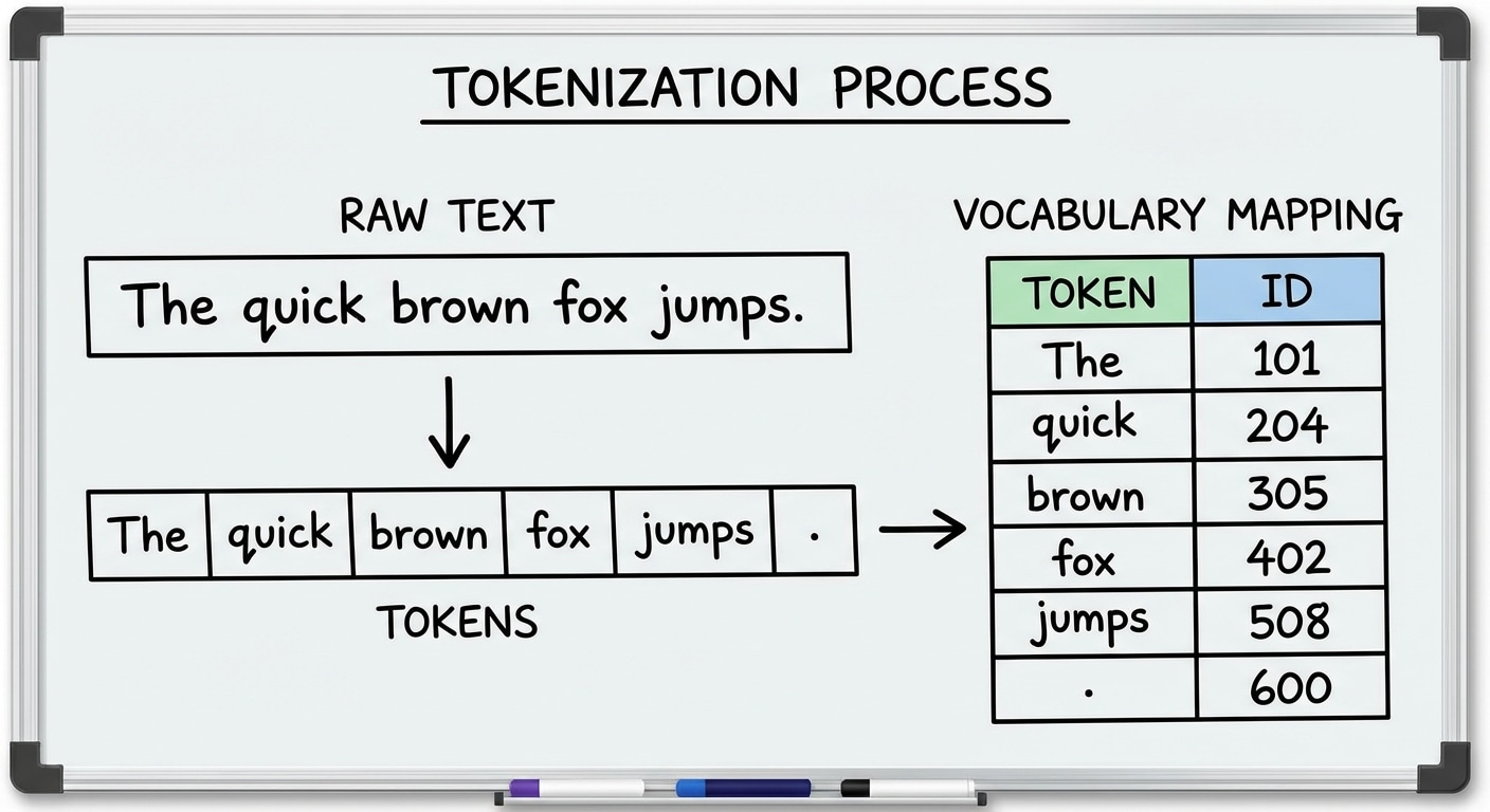
Before AI can process text, it must be split into tokens – the fundamental units the model works with. Tokenization strategy significantly impacts model performance, vocabulary size, and ability to handle rare or novel words. Getting it right matters more than many realise.

Word-level tokenization splits on whitespace, creating intuitive tokens but massive vocabularies. Unknown words become impossible to handle. Character-level uses each character as a token, handling any text but losing word-level semantics and creating very long sequences.

Subword tokenization like BPE and WordPiece offers the best of both worlds. Common words remain whole while rare words split into meaningful subwords. The vocabulary stays manageable at 32K-100K tokens while handling novel words by decomposition.

Modern tokenizers also handle special tokens for model control: beginning and end of sequence markers, padding tokens, and special separators. Understanding tokenization helps debug model behaviour – sometimes strange outputs trace back to unexpected token boundaries.

Word Embeddings Explained

Embeddings

Word Embeddings: Meaning in Vectors

Word embeddings convert discrete tokens into dense vectors where semantic similarity corresponds to geometric proximity. This representation enables neural networks to understand that king and queen are related, or that Paris relates to France as Rome relates to Italy.

Early methods like Word2Vec learn embeddings by predicting context from words or vice versa. GloVe factors word co-occurrence matrices for global statistics. These static embeddings assign one vector per word regardless of context, missing nuances like bank meaning riverbank versus financial institution.

Contextual embeddings from BERT and GPT solved this limitation. The same word gets different representations based on surrounding context. This dynamic understanding dramatically improved performance on tasks requiring disambiguation and nuanced comprehension.

Embeddings reveal learned structure through vector arithmetic. The classic example: king minus man plus woman equals queen. These relationships emerge unsupervised from training data, demonstrating that neural networks discover meaningful semantic structure without explicit guidance.

Self-Attention Mechanism Explained

Attention

Self-Attention: The Core of Transformers

Self-attention allows each element in a sequence to attend to all other elements, capturing relationships regardless of distance. This mechanism revolutionized NLP by replacing recurrence with parallelisable attention operations that model long-range dependencies more effectively.

For each token, three vectors are computed: Query (what am I looking for), Key (what do I contain), and Value (what information do I provide). Attention weights come from the dot product of Query and Key, normalised by softmax. These weights determine how much each token contributes to the output.

Multi-head attention runs multiple attention mechanisms in parallel, each learning to focus on different relationship types. One head might capture syntactic dependencies while another focuses on semantic similarity. Concatenating and projecting results combines these perspectives.

The attention mechanism enables remarkable capabilities in language models. A model can understand that a pronoun refers to a noun mentioned paragraphs earlier, or that a technical term definition from the context applies throughout. This contextual understanding underpins modern LLM performance.

LSTM Networks Explained

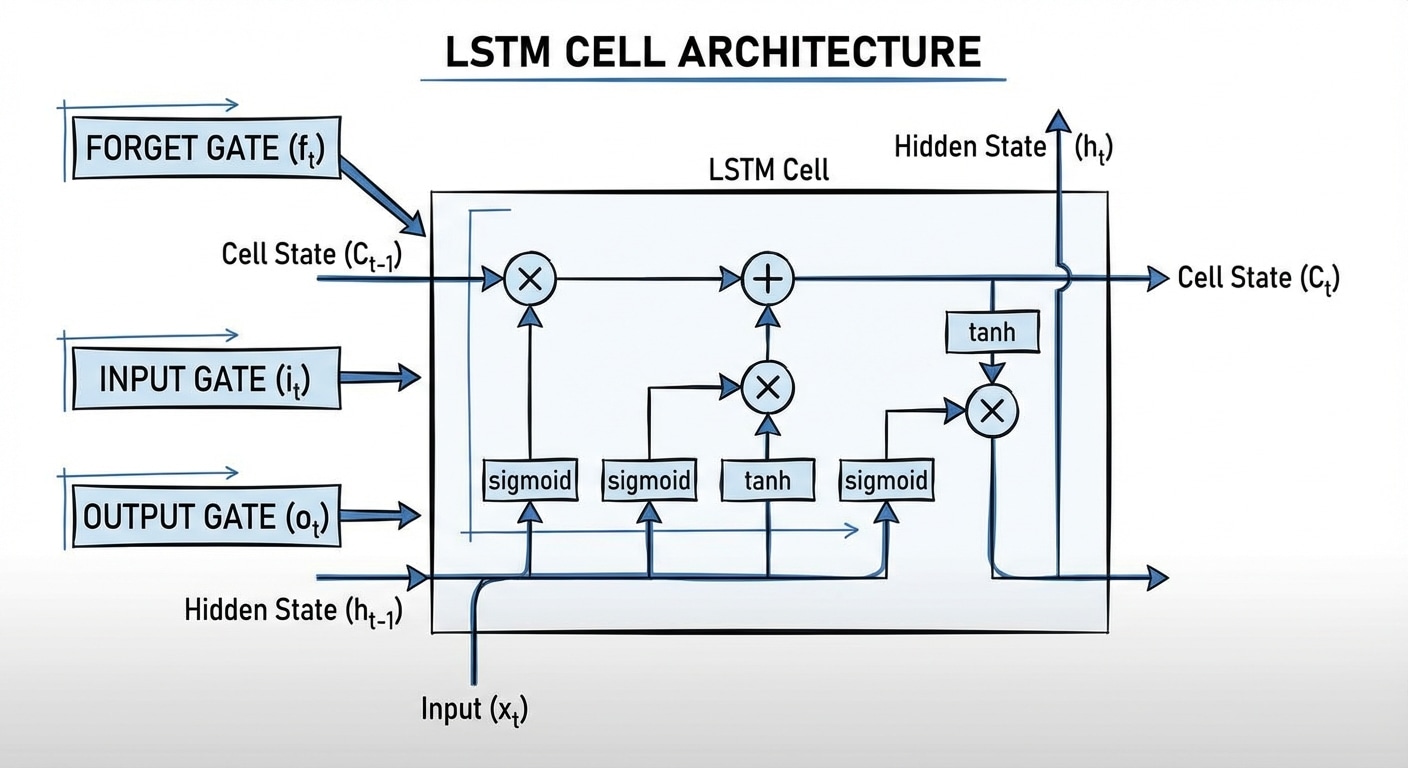
LSTM Cell Architecture Diagram

Introduction: The Power of LSTMs

The Long Short-Term Memory (LSTM) network is a specialised kind of Recurrent Neural Network (RNN) architecture, designed specifically to solve the problem of vanishing gradients that plagues traditional RNNs when dealing with long sequences of data.

While standard RNNs struggle to retain information from many steps ago, LSTMs are engineered with a dedicated Cell State (Ct)—often called the “conveyor belt”—that runs straight through the network. This Cell State is regulated by three distinct, multiplicative gates (Forget, Input, and Output) that learn to selectively remember or forget information, allowing the network to capture and utilise long-term dependencies in sequential data like text, speech, and time series. The mathematical equations below illustrate how these gates precisely control the flow of both long-term memory (Ct) and short-term output (ht).


LSTM Cell Architecture Equations

This breakdown translates the LSTM diagram into its corresponding mathematical equations, showing exactly how the inputs (xt, ht-1, Ct-1) are processed to generate the outputs (ht, Ct).

The σ symbol represents the Sigmoid function, and W and b represent the weight matrices and bias vectors learned during training.

1. The Gates (Control)

The first step is calculating the three gates, each using the current input (xt) and the previous hidden state (ht-1) and applying a sigmoid function (σ):

A. Forget Gate (ft):

ft = σ(Wf · [ht-1, xt] + bf)

Purpose: Decides which information to forget from the old cell state (Ct-1).

B. Input Gate (it):

it = σ(Wi · [ht-1, xt] + bi)

Purpose: Decides which values to update in the cell state.

C. Candidate Cell State (ᶜt):

t = tanh(WC · [ht-1, xt] + bC)

Purpose: Creates a vector of potential new values that could be added to the cell state.

2. Cell State Update (The Memory)

The Cell State (Ct) is the core memory of the LSTM, updated by combining the old memory and the new candidate memory:

Ct = ft ∗ Ct-1 + it ∗ ᶜt

  • The term ft * Ct-1 implements the forgetting mechanism: the old memory Ct-1 is scaled down by the Forget Gate ft.
  • The term it * ᶜt implements the input mechanism: the new candidate information ᶜt is scaled by the Input Gate it.
  • These two parts are then added to create the new long-term memory, Ct.

3. Hidden State Output (The Prediction)

The Hidden State (ht) is the final output of the cell at this time step. It is based on the new Cell State, filtered by the Output Gate:

A. Output Gate (ot):

ot = σ(Wo · [ht-1, xt] + bo)

Purpose: Decides which parts of the (squashed) Cell State will be exposed as the Hidden State.

B. Final Hidden State (ht):

ht = ot ∗ tanh(Ct)

  • The new Cell State Ct is passed through tanh to bound the values between -1 and 1.
  • The result is then element-wise multiplied by the Output Gate ot to produce the final short-term memory and output vector, ht.

Conclusion: The Importance of Selective Memory

The LSTM architecture, as described by these equations, fundamentally improved the capability of recurrent neural networks to model complex dependencies over long sequences. By using three learned, multiplicative gates to regulate the flow into and out of the Cell State, the LSTM is able to maintain a stable, uncorrupted memory path, overcoming the practical limitations of standard RNNs.

This innovation has made LSTMs essential tools in areas requiring deep contextual understanding, leading to breakthroughs in speech recognition, machine translation, and text generation, before the wider adoption of the Transformer architecture.

Next Steps

Interested in a simpler alternative? Check out the GRU (Gated Recurrent Unit), which combines the forget and input gates into a single update gate—achieving similar performance with fewer parameters. For cutting-edge sequence modeling, explore how Transformers use attention mechanisms to process entire sequences in parallel, bypassing recurrence altogether.