Author: David Saliba

Models plan; code executes. The loop is non-negotiable: propose an action, run it, feed the result back, repeat until done. What is negotiable is where the loop runs – in your service, or inside the inference provider’s runtime behind a single API call.

The Goal Gate

Both patterns share one thing: a rule that says “we are done.” Without it the agent loops forever. In code it looks like this:

// Three ways to terminate a loop:

// 1. Model returned a final answer (no tool calls requested)
if (!res.tool_calls?.length) return res.content;

// 2. Hard step budget - never let open-ended tasks burn silently
if (step >= MAX_STEPS) throw new Error("step budget exceeded");

// 3. Judge call - a rules check or small classifier says the
//    original question is satisfied even if the model wants more
if (await judge.isSatisfied(originalQuery, accumulatedAnswer)) return;

Local and managed loops differ in who runs that gate – your for loop or the provider runtime – not in whether it exists.

Local Loop: Your Code Owns Every Hop

Example: “What’s the status of order 8842?”

// ── HOP 1: send user message to model ──────────────────────────────
const hop1 = await llm.chat({
  messages: [
    { role: "system", content: "Use lookup_order when needed." },
    { role: "user",   content: "What's the status of order 8842?" }
  ],
  tools: [lookupOrderSchema]
});
// Model does NOT answer yet - it requests a tool:
// { content: null, tool_calls: [{ name: "lookup_order", arguments: { order_id: "8842" } }] }

// ── YOUR CODE RUNS THE TOOL (not the LLM) ──────────────────────────
const result = await db.query(
  "SELECT status, carrier, eta FROM orders WHERE id = $1",
  ["8842"]
);
// { status: "shipped", carrier: "DHL", eta: "2026-06-26" }

// ── HOP 2: feed the result back, get the final answer ──────────────
const hop2 = await llm.chat({
  messages: [
    ...previousMessages,
    { role: "tool", tool_call_id: hop1.tool_calls[0].id,
      content: JSON.stringify(result) }
  ],
  tools: [lookupOrderSchema]
});
// { content: "Order 8842 shipped via DHL, arrives 26 June.", tool_calls: [] }

// ── GOAL GATE: tool_calls empty -> exit loop, send reply to user ───

One user turn. Two LLM round-trips. One DB query. Log all three latency contributions separately – never lump them into a single “response time” figure.

Example: Multi-tool research (three hops, one visible reply)

User: Compare our refund policy with what competitor X published last month.

Two messages in the chat UI. Three internal hops:

1. Model requests fetch_url(competitorPricingURL). Your scraper runs and returns markdown.
2. Model requests search_knowledge_base("refund policy"). Your vector DB returns a chunk.
3. Model synthesises both results. No further tool calls. Goal gate opens.

// Each hop gets its own metric - this is what tells you which one is slow:
metrics.record("llm_hop1_ms",    hop1ElapsedMs);
metrics.record("tool_fetch_url_ms", fetchElapsedMs);
metrics.record("tool_search_kb_ms", searchElapsedMs);
metrics.record("llm_hop2_ms",    hop2ElapsedMs);

The full local runner

async function runAgent(messages, tools, maxSteps = 8) {
  for (let step = 0; step < maxSteps; step++) {
    const res = await llm.chat({ messages, tools });

    // Goal gate: model returned a final answer.
    if (!res.tool_calls?.length) return res.content;

    // Execute every requested tool locally, append results to context.
    for (const call of res.tool_calls) {
      const out = await executeLocally(call);  // your code, your network, your logs
      messages.push({ role: "tool", tool_call_id: call.id,
                      content: JSON.stringify(out) });
    }
  }
  // Goal gate never triggered inside the step budget.
  throw new Error("max steps reached");
}

Managed Loop: Provider Runs the Inner Cycle

Same logical loop, but the provider runs it. Your application sends one request; the provider calls the model, dispatches tools, feeds results back, and returns only when its internal goal gate fires.

Example: "What's the status of order 8842?" (managed)

// ── YOUR APPLICATION: one call ─────────────────────────────────────
const res = await llm.chat({
  messages: [
    { role: "system", content: "You help with orders." },
    { role: "user",   content: "What's the status of order 8842?" }
  ],
  tools: [{
    type: "mcp",
    server_url: "https://tools.example.com/mcp",  // must be publicly reachable
    allowed_tools: ["lookup_order"]
  }]
});
// Your code blocks here. Provider is running the loop internally.
// res.content == "Order 8842 shipped via DHL, arrives 26 June."

// ── WHAT HAPPENED INSIDE (only visible if you enable tracing) ──────
// [1] Model: tool_call lookup_order("8842")
// [2] Provider: connects to MCP server, runs tool, gets JSON
// [3] Model: synthesises final reply
// [4] Goal gate: no further tool calls -> return to client

Same reply. Different accountability surface. Your MCP server must be publicly reachable from provider egress IPs. Empty tool results never pass through your code, so handle them with a system-prompt rule:

// Add to system prompt for any managed-tool agent:
"If a tool returns no data or an error, say so explicitly.
 Do not infer or invent the answer."

Example: Web search agent (managed, serial tools)

// Your app:
const res = await llm.chat({
  messages: [{ role: "user",
    content: "Summarise Kubernetes networking changes in the last six months." }],
  tools: [{ type: "web_search", max_uses: 4 }]
});
// Provider internally: search -> search -> fetch -> synthesise
// User sees one reply after 3-8 seconds.
// Your logs show one API call. Provider traces show four hops.

Side-by-Side: Same Chat, Different Plumbing

Latency: Count Every Hidden Hop

// Case 1: local tool cost ranges
// - in-process lookup:       < 1 ms
// - local MCP over stdio:    ~1 ms (warm process)
// - remote HTTP API:         50-300+ ms
// - cold MCP server boot:    seconds on first request

// Case 2: managed loop budget check - do this before committing
const budgetMs     = 800;   // acceptable TTFT for chat UX
const modelMs      = 350;   // per inner LLM call
const innerLlmCalls = 2;    // typical for one tool use
const toolMs       = 280;   // per tool round-trip

const totalMs = modelMs * innerLlmCalls + toolMs;
// 980ms - over budget.
// Fix: keep latency-sensitive tools local, parallelise, or reduce max_uses.

// Case 3: silent failure guard (managed mode)
// Model receives an empty tool result and may hallucinate a confident answer.
// There is no if/catch in your code path - the model is your only filter.
// System prompt rule is the guard:
"If any tool returns empty or an error, say so. Do not invent an answer."

Failures You Still Own in Managed Mode

// WRITE IDEMPOTENCY
// Read tools retry cleanly. Write tools need dedup keys:
const orderPayload = {
  idempotency_key: crypto.randomUUID(),  // provider may retry internally
  ...orderData
};

// NETWORK REACHABILITY
// Tools on private networks cannot move to managed without a proxy.
// Test before cutover:
curl -I https://tools.example.com/mcp  // must respond from provider egress IPs

// ALERT GRANULARITY - split these, they have different fixes:
// - provider_latency_p95
// - mcp_cold_start_ms
// - model_quality_degradation (separate alert, separate runbook)

When to Stay Local

• During development - you need per-hop logs and breakpoints at the tool boundary.
• Sub-second chat or voice UX where managed overhead is user-visible.
• Tools on private networks or requiring local session state.
• Custom goal gates: compliance judges, human-in-the-loop approval, or termination logic the provider runtime cannot implement.

When Managed Makes Sense

• Standard search and retrieval where you do not want to run your own search infrastructure.
• Many separate agents sharing one MCP tool surface.
• Tool credentials that should not live in application repositories.
• Teams that prefer paying with a tracing subscription rather than maintaining a loop runner.

Migration Path

1. Build local first. Log tool name, argument size, latency, result size per hop from day one.
2. Classify tools: read vs write, local vs remote, latency-sensitive vs batch-tolerant.
3. Move read-only, tolerant tools to managed first. Keep write tools local until idempotency keys and retry semantics are confirmed.
4. Enable provider tracing before cutover and compare inner-hop counts against your local logs. Divergence means something changed.

Swarms to Keep an Eye On

This covers the single-agent loop: one context window, serial hops. When tasks decompose into parallel research lanes, or you need orchestrator-worker topologies and peer handoffs, you are in multi-agent territory with different cost structures and failure modes. For the full evolution map - single-shot LLM through ReAct loop, agent stack, orchestrator swarms, and a 2026 watchlist - read the companion piece:

From Chat Completion to Agent Swarms: How Loop Architecture Evolved

What to Check Right Now

• Draw your loop on paper with numbered hops and the goal gate labelled. If you cannot draw it, your production agent is opaque.
• Split latency metrics: model time vs tool time per user-visible reply. An aggregate figure hides which hop is slow.
• Measure MCP cold-start from a fresh process - that is what a first-morning user experiences.
• Audit write tools for idempotency keys before moving any to managed mode.
• Tool count check: past ~25 tools, evaluate deferred schema loading to reduce input token cost.

Managed execution shrinks code; it does not shrink accountability. The chat looks the same to the user either way. What changes is whether you can see the loops between their question and the answer - and whether you find out about failures before or after they do.

nJoy 😉

Your RAG pipeline is lying to you. Not maliciously, of course, but with the quiet confidence of a student who memorised the textbook’s index but never read a chapter. You feed it documents, it chunks them, embeds them, and when you ask a question it retrieves whichever chunks look “sort of similar” and hopes the LLM can stitch together a coherent answer. Sometimes it works. Sometimes it tells you Tokyo has 36 million people because it averaged two contradictory chunks. And you have no way to know which answer is real, because Vector RAG has no concept of “real”. It only knows “similar”. Context graphs are what happens when you decide similarity is not enough, and you want your AI to actually understand the relationships between things. TrustGraph just shipped a demo that shows exactly what that looks like in practice, and it is worth paying attention to.

What Context Graphs Actually Are (and Why They Are Not Just Knowledge Graphs With a Rebrand)

A context graph is a knowledge graph that has been specifically engineered for consumption by AI models. That sentence sounds like marketing, so let us unpack it. A traditional knowledge graph stores millions of entities and relationships, optimised for human querying and data warehousing. Brilliant for analysts running SPARQL queries. Terrible for an LLM with a context window that starts forgetting things after a few thousand tokens.

Context graphs solve this by dynamically extracting focused subgraphs based on query relevance. Instead of dumping the entire graph into the prompt, you extract only the entities and relationships that matter for this specific question, scored by relevance, annotated with provenance, and formatted to minimise token waste. TrustGraph’s own documentation claims a 70% token reduction in their structured-versus-prose comparison. That number is plausible for the specific example they show (a simple entity lookup), but it is a vendor benchmark, not an independent evaluation, and the savings will vary dramatically depending on query complexity, graph density, and how much context the LLM actually needs.

“Context graphs are knowledge graphs specifically engineered and optimized for consumption by AI models. They extend traditional knowledge graphs by incorporating AI-specific optimizations like token efficiency, relevance ranking, provenance tracking, and hallucination reduction.” — TrustGraph, Context Graphs Guide

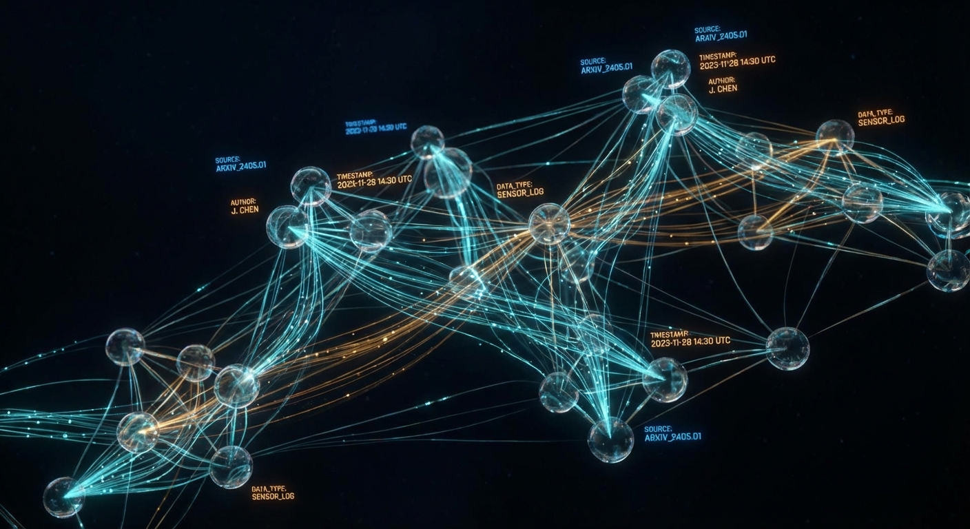
Think of the distinction this way. A knowledge graph is your entire library. A context graph is the specific stack of books your librarian pulls when you ask a particular question, each one bookmarked at the relevant page, with a note explaining why it was selected. The librarian remembers which shelf each book came from, when it was last updated, and how confident she is that the information is still correct. That is what provenance tracking and relevance scoring give you.

Here is the structural difference in compact form:

// Traditional knowledge graph: everything, all at once
{
  entities: [/* millions */],
  relationships: [/* tens of millions */]
}

// Context graph: query-specific, AI-optimised
{
  query: "Who leads TechCorp?",
  entities: [
    { name: "Alice Johnson", role: "CEO", relevance: 0.95 },
    { name: "TechCorp", industry: "Enterprise Software", relevance: 0.92 }
  ],
  relationships: [
    { from: "Alice Johnson", to: "TechCorp", type: "leads", relevance: 0.90 }
  ],
  metadata: { tokensUsed: 350, confidenceScore: 0.94, sources: ["hr_database"] }
}

The verbose natural-language equivalent of that context graph would cost 150 tokens. The structured version costs 45. Same information, a third of the price. As Martin Kleppmann writes in Designing Data-Intensive Applications, the way you structure your data determines what questions you can efficiently answer. Context graphs are structured specifically to answer LLM questions efficiently.

The TrustGraph Demo: London Pubs, Craft Beer, and Why Semantics Matter

The video “Context Graphs in Action” by TrustGraph co-founders Daniel Davis and Mark Adams is a 27-minute live demo. No slides. No marketing deck. They built a context graph from data about London pubs, restaurants, and event spaces, then demonstrated something deceptively simple that reveals the entire value proposition of this technology.

They asked two questions that any human would consider identical:

1. “Where can I drink craft beer?”
2. “Can you recommend a pub which serves craft beer?”

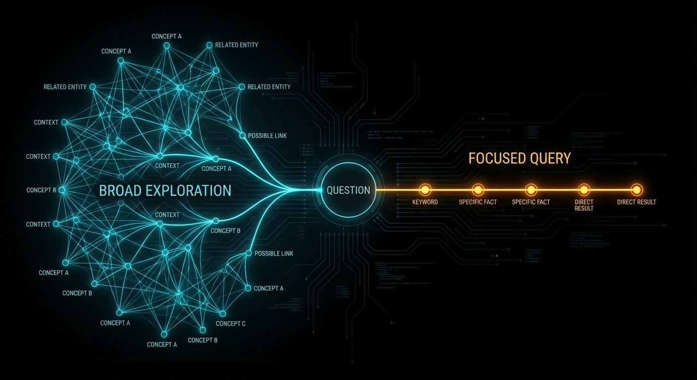
Both questions returned the same answer. But when they expanded the explainability trace, the paths through the graph were completely different. The first question, being open-ended, pulled in concepts from beer gardens, festivals, events, bars, cafes, and dozens of other venue types. The second question, with the word “pub” constraining the search, produced a far narrower traversal. The grounding concepts were different. The subgraph was different. The reasoning path was different. Only the final answer happened to converge.

This is the central insight the demo drives home: two questions that feel identical to a human are semantically distinct to a machine, and context graphs let you see exactly how and why. As Daniel puts it with characteristic bluntness: “If you ask a stupid question, you might get a stupid response.” The explainability trace lets you work backwards from a bad answer and determine whether the fault lay with the query, the data, or the retrieval path.

What the Workbench Actually Shows

The demo walks through TrustGraph’s Workbench interface (accessible at localhost:8888 after deployment). Here is what they demonstrated:

• Document ingestion: Plain text and PDF documents about London venues are uploaded through the Library page and processed through a GraphRAG flow. TrustGraph chunks the documents, extracts entities and relationships, generates vector embeddings, and builds the knowledge graph automatically.
• Vector search entry points: Searching for “Bermondsey” returns semantically similar terms. Clicking a result reveals the fabric of the graph: Bermondsey tube station connects to the Jubilee line, which has a type “transport line”. You can navigate relationships in 3D space.
• 3D graph visualisation: Interactive three-dimensional exploration of graph nodes and edges. Not intended for end users (Daniel jokes it would “send everybody over the edge insane”), but invaluable for understanding graph structure during development.
• Explainability traces: Every query records a full reasoning trace. You can see: the original query, which concepts were extracted, which graph nodes matched, which edges were traversed, why each piece of evidence was selected (with the LLM’s reasoning), and the final synthesis. All traceable back to source documents.
• Source provenance: Every fact in the graph links back to the specific document chunk it was extracted from. You can verify: where did this information come from? When was it ingested? Is it out of date? Do we trust this source?

The Ontology Question

Mark Adams demonstrates both approaches: schema-free extraction (GraphRAG) where the LLM discovers relationships freeform, and ontology-driven extraction (OntologyRAG) where a predefined schema forces precision. For the London venues demo, the ontology defines classes like “atmosphere” (cozy, creative, community spirit), “city”, “neighbourhood”, “event”, and constrains the relationships the graph will accept.

The result with ontologies is significantly more precise. Without an ontology, the LLM sometimes creates duplicate relationships with different names for the same concept. With an ontology, you control the vocabulary, and precision goes up. As Mark explains: “We force it into a much more precise structure.”

TrustGraph sits firmly in the RDF ecosystem rather than the property graph world (Neo4j and similar). The rationale: RDF supports reification (attaching metadata to edges themselves), multi-language representations, and the OWL/SKOS ontology standards natively. These features are essential for explainability and provenance tracking.

But let us be honest about the trade-offs. RDF comes with real costs. SPARQL is notoriously harder to learn than Cypher (Neo4j’s query language). OWL ontologies require domain experts to design and maintain, and they become a governance burden as your data evolves. Property graphs with Neo4j or Memgraph are simpler to reason about, faster for most traversal patterns, and have much larger developer ecosystems. TrustGraph’s choice of RDF is defensible for provenance-heavy enterprise use cases, but it is not the only valid architecture, and for many teams a property graph with LangGraph or LlamaIndex’s knowledge graph module will be simpler to operate and good enough.

The Broader Landscape: TrustGraph Did Not Invent This

Before we go further, some necessary context. The idea of using knowledge graphs to ground LLM responses is not new, and “context graph” is not a category that TrustGraph created from scratch. It is a refined evolution of work that has been shipping in production since late 2024.

Microsoft GraphRAG published the foundational “From Local to Global” paper in April 2024, introducing community-based summarisation of knowledge graphs for query-focused retrieval. Their approach extracts entities and relationships, clusters them into hierarchical communities using the Leiden algorithm, then pre-generates summaries at each level. It is open source, integrates with Neo4j, and has an Azure solution accelerator. Microsoft also shipped LazyGraphRAG (November 2024) to address the cost problem, and BenchmarkQED (June 2025) for automated RAG evaluation.

Neo4j + LangChain/LangGraph is arguably the most widely deployed graph RAG stack in production today. Neo4j’s property graph model with Cypher queries is simpler to learn than SPARQL, has a massive developer community, and integrates directly with LangChain’s retrieval chains. For teams already running Neo4j, adding graph-enhanced RAG requires no new infrastructure.

LlamaIndex Knowledge Graphs provides a Python-native graph RAG pipeline that works with Neo4j, Nebula Graph, and others. It handles entity extraction, graph construction, and hybrid vector+graph retrieval with significantly less operational complexity than a full RDF stack.

What TrustGraph adds to this landscape is specifically the combination of RDF-native ontology support, built-in explainability traces, portable context cores, and multi-model storage (Cassandra, Qdrant, etc.) in a single open-source platform. These are genuine differentiators for provenance-heavy enterprise use cases. But if you do not need ontology enforcement or full reasoning traces, the simpler alternatives above will get you 80% of the benefit at 20% of the operational complexity.

Where Vector RAG Falls Apart (and Context Graphs Save You)

Vector RAG seemed like the answer to everything when embeddings first became cheap. Embed your documents, find similar chunks, feed them to the LLM. Fast, simple, works for demos. Then you deploy it in production and discover the failure modes.

Case 1: The Averaging Problem

You embed two documents. One says “Tokyo’s population is 37.4 million.” The other says “Tokyo has about 35 million people.” Both are semantically similar to the query “What is Tokyo’s population?” The LLM sees both chunks and generates something in between. Maybe 36 million. Confidently wrong.

// Vector RAG retrieval for "What is Tokyo's population?"
chunk_1: "Tokyo's population is 37.4 million" (similarity: 0.94)
chunk_2: "Tokyo has about 35 million people" (similarity: 0.92)
// LLM output: "Tokyo has approximately 36 million people" -- wrong

// Context graph retrieval
node: Tokyo { population: 37400000, source: "UN World Population Prospects 2024",
              confidence: 1.0, lastVerified: "2024-07-01" }
// LLM output: "Tokyo's population is 37.4 million" -- correct, sourced, verifiable

A graph stores one value. The correct value. With a source and a timestamp. No ambiguity, no averaging, no hallucination.

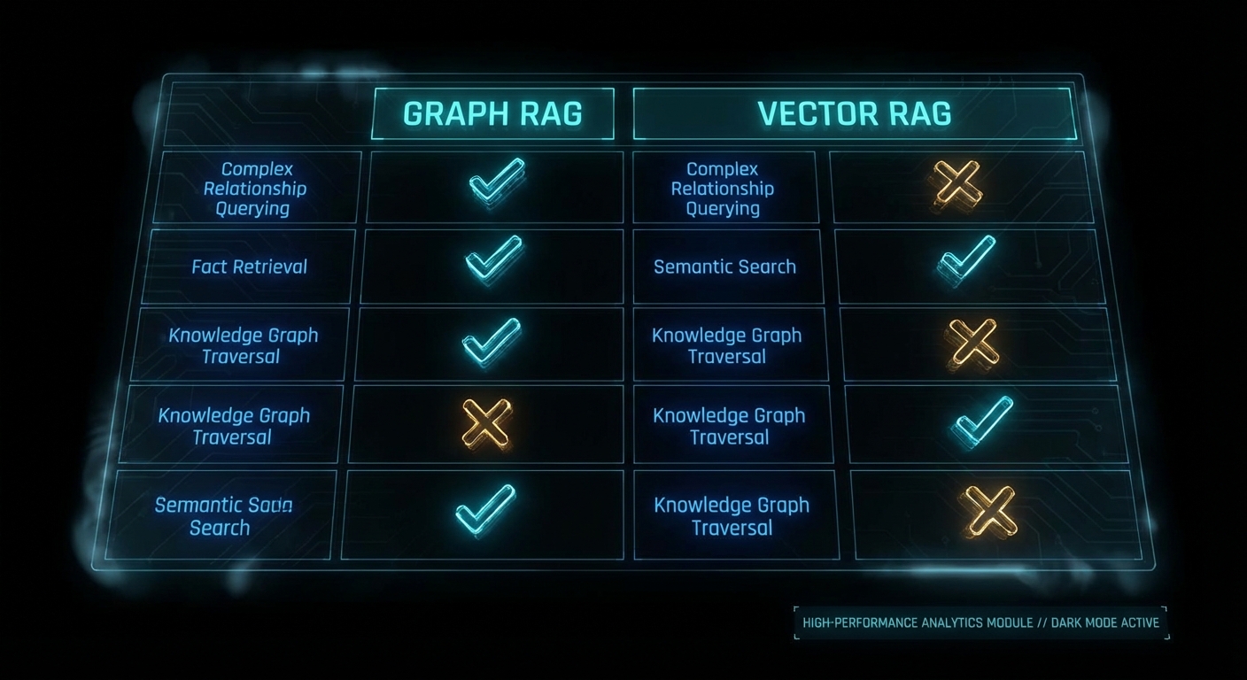
Case 2: The Multi-Hop Blindness

Ask Vector RAG: “How does climate change affect AI research funding?” It needs to traverse: climate change affects government priorities, which influence research funding allocation, which supports AI research. Each of those facts lives in a different document. Vector RAG retrieves chunks that are individually similar to the question but cannot connect them into a reasoning chain.

// Vector RAG: retrieves 3 chunks that mention some of these concepts
// but cannot chain: climate -> govt priorities -> funding -> AI research
// Result: vague, hedge-filled answer

// GraphRAG: traverses the reasoning path
climate_change --[affects]--> government_priorities
government_priorities --[influences]--> research_funding
research_funding --[supports]--> ai_research
// Result: specific, grounded answer with full provenance chain

Independent benchmarks from Iterathon’s 2026 enterprise guide report GraphRAG achieving 83-87% accuracy on complex multi-hop queries versus Vector RAG’s 68-72%. Microsoft’s own evaluation found GraphRAG improved comprehensiveness by 26% and diversity by 57% over standard vector retrieval. These numbers are promising, but a caveat: most published benchmarks come from vendors or researchers with a stake in the outcome. Independent, apples-to-apples comparisons across Microsoft GraphRAG, Neo4j + LangChain, LlamaIndex, and TrustGraph on the same dataset remain conspicuously absent from the literature.

Case 3: The Lost-in-the-Middle Catastrophe

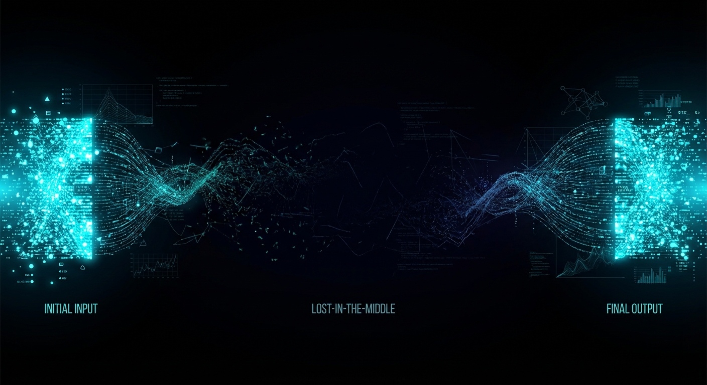
Here is the one that should worry every engineer relying on long context windows as a substitute for proper retrieval. Research by Liu et al. at Stanford demonstrated that LLMs consistently fail to use information placed in the middle of long contexts, even when the context window is enormous.

“Language models exhibit significantly degraded performance when relevant information is positioned in the middle of long contexts, even for models explicitly designed for long-context processing.” — Liu et al., “Lost in the Middle: How Language Models Use Long Contexts”, TACL 2024

TrustGraph’s own testing confirms this pattern holds across models. Chunks of 1,000 tokens extracted 2,153 graph edges. Chunks of 8,000 tokens extracted only 1,352. That is a 59% increase in extracted knowledge just from chunking smaller, using only 4% of the available context window. At 500 tokens, the system extracted 2,975 edges, a 120% improvement over 8,000-token chunks. This pattern held across eight models from six providers: Claude, Gemini, Mistral, Cohere, Llama, and others.

Long context windows do not work. Not because the models are bad, but because the transformer attention mechanism dilutes focus as token count rises. This appears to be inherent to the architecture itself. Context graphs sidestep the problem entirely: instead of cramming everything into a massive context, you extract a small, focused, structured subgraph. The LLM gets exactly what it needs and nothing else.

How to Actually Deploy This: From Zero to Context Graph

TrustGraph is open source (Apache 2.0) and deploys via Docker Compose in minutes. Here is the real pipeline, not the marketing version:

Step 1: Configure and Deploy

# Install and configure TrustGraph
npx @trustgraph/config

# Interactive prompts:
# ? Select your LLM provider: Anthropic / OpenAI / Google / Mistral / Ollama
# ? Select deployment target: Docker / Kubernetes / Minikube
# Generates docker-compose.yaml and INSTALLATION.md

# Deploy
docker compose up -d

# Workbench available at http://localhost:8888
# Grafana monitoring at http://localhost:3000

Step 2: Ingest Documents and Build the Graph

# Create a collection
tg-set-collection \
  -n "Company Docs" \
  -d "Internal documentation" \
  company-docs

# Add a document
tg-add-library-document \
  --name "Security Policy 2025" \
  --id doc-security-2025 \
  --kind application/pdf \
  documents/security-policy.pdf

# Create a GraphRAG flow (no ontology needed)
tg-start-flow \
  -n graph-rag \
  -i security-graphrag \
  -d "Security document knowledge extraction"

# Process the document
tg-start-library-processing \
  --flow-id security-graphrag \
  --document-id doc-security-2025 \
  --collection company-docs

Step 3: Query With Explainability

# GraphRAG query with full provenance
tg-invoke-graph-rag \
  -f security-graphrag \
  -C company-docs \
  -q "What are our top cybersecurity vulnerabilities?"

# Or via the REST API
curl -X POST http://localhost:8001/api/invoke/graph-rag \
  -H "Content-Type: application/json" \
  -d '{
    "flow-id": "security-graphrag",
    "collection": "company-docs",
    "query": "What are our top cybersecurity vulnerabilities?",
    "max-entities": 50,
    "relevance-threshold": 0.7,
    "include-provenance": true
  }'

The TypeScript client library (@trustgraph/client) provides WebSocket-based real-time communication for building production UIs. Python and CLI interfaces are also available.

Step 4: Add Ontologies for Precision (Optional but Recommended)

# Upload an OWL ontology
cat domain-ontology.owl | tg-put-config-item \
  --type ontology \
  --key security-ontology \
  --stdin

# Create an OntologyRAG flow
tg-start-flow \
  -n onto-rag \
  -i security-onto-rag \
  -d "Ontology-driven security knowledge extraction"

# Process with ontology enforcement
tg-start-library-processing \
  --flow-id security-onto-rag \
  --document-id doc-security-2025 \
  --collection company-docs

The Unglamorous Reality: What Graph RAG Actually Costs You

Every GraphRAG vendor demo shows the happy path. Here is what they leave out.

Ingestion Is Expensive and Slow

Building a knowledge graph requires running every document chunk through an LLM for entity and relationship extraction. This is not free. Microsoft’s original GraphRAG architecture dedicates roughly 75% of total indexing cost to graph extraction alone. One production deployment reported $33,000 in indexing costs for a large dataset before a single query was run. A 10,000-document corpus that costs under $5 to embed in a vector database costs $50-200 to process through a GraphRAG pipeline. For context: that is a 10-40x cost multiplier at ingestion time.

Entity Resolution Is the Silent Killer

When your LLM extracts entities from thousands of documents, it will create duplicates. “IBM”, “International Business Machines”, “IBM Corp”, and “Big Blue” are all the same entity. If your entity resolution accuracy drops below roughly 85%, the errors compound exponentially through multi-hop queries. At 85% accuracy with 5 hops, fewer than half your answers remain trustworthy (0.85^5 = 44%). This is not a theoretical problem; it is the most common failure mode in production GraphRAG systems, and neither TrustGraph nor anyone else has fully solved it.

Ontology Maintenance Is a Governance Burden

TrustGraph’s OntologyRAG produces more precise graphs, no question. But someone has to design that ontology, maintain it as your domain evolves, and ensure new documents conform to the schema. In practice, this means a dedicated knowledge engineer or a committee that reviews and updates the ontology quarterly. For organisations that already struggle to maintain a data dictionary, adding OWL ontology governance is a non-trivial ask.

Three Indexes, Three Consistency Problems

Production graph RAG requires keeping three synchronized stores: a graph index for structural traversal, a vector index for semantic similarity, and often a text index for full-text search. Every document addition, update, or deletion must propagate across all three and trigger entity resolution re-evaluation. This is, bluntly, a data engineering nightmare that most demos conveniently skip.

Extraction Hallucinations Are Real

The LLM that extracts entities and relationships from your documents will hallucinate some of them. It will invent relationships that do not exist in the source text, misattribute properties, and occasionally create phantom entities. These extraction hallucinations then become “facts” in your knowledge graph, where they are retrieved with the same confidence score as legitimate data. Garbage in, graph out. Every production deployment needs a quality assurance pipeline to catch extraction errors, and most teams underestimate this effort.

Query Latency Is Not Milliseconds

Vector search returns results in single-digit milliseconds. Graph RAG queries involve: vector lookup to find entry points, graph traversal across multiple hops, LLM-based relevance scoring of candidate edges, subgraph assembly, and finally LLM generation. End-to-end latency is typically 2-15 seconds depending on graph size and traversal depth. For interactive applications where users expect sub-second responses, this is a hard constraint that no amount of clever engineering fully eliminates.

When Context Graphs Are Essential (Real Use Cases)

Context graphs are not a universal hammer. They are a precision instrument for specific categories of problem. Here is where they earn their keep:

• Financial compliance and audit: A financial analyst querying regulatory exposure across multiple counterparties needs multi-hop reasoning across hundreds of documents. Every answer must be traceable to source documents for regulatory compliance. SowFin, a corporate finance company, uses TrustGraph to bring accurate, explainable insights to corporate finance.
• Security operations: Huntbase uses TrustGraph to build Context Cores for SecOps, where AI hallucinations in threat detection are not just inconvenient but dangerous. Cybersecurity requires connecting events, metadata, and threat indicators across thousands of log entries with full provenance.
• Medical and clinical research: Clinical informaticists analysing treatment interactions across patient comorbidities need graph traversal to connect drugs, conditions, contraindications, and outcomes across multiple clinical databases. Approximate similarity search is not acceptable when lives are involved.
• Supply chain management: Tracing component dependencies multiple tiers deep requires genuine relationship traversal. “Which suppliers are affected if factory X in Shenzhen shuts down?” demands multi-hop graph queries that Vector RAG simply cannot do.
• Legal document analysis: Connecting clauses across contracts, precedents across cases, and regulations across jurisdictions. Every connection must be verifiable and traceable.
• Enterprise knowledge management: The “monograph” approach (a single unified graph across all your organisation’s knowledge) enables discovery of relationships across departments and domains that siloed systems miss. This is not unique to TrustGraph; any sufficiently connected knowledge graph achieves this, whether built with Neo4j, Microsoft GraphRAG, or TrustGraph.

When Context Graphs Are Overkill (Be Honest With Yourself)

Now for the part that most GraphRAG vendors would rather you did not read. Context graphs are genuinely overkill for a significant number of common AI use cases. Using one when you do not need one is like hiring a structural engineer to hang a picture frame.

• Small datasets that fit in context: If your entire corpus is under 50 pages (roughly 40,000 tokens), skip RAG entirely. Stuff it all into the prompt. It costs $0.01 per query versus $0.05 for a RAG pipeline, deploys in a day versus four weeks, and the LLM can attend to all of it directly. No chunking, no embeddings, no graph. Simple prompt engineering wins.
• General knowledge queries: Questions the LLM already knows the answer to (world history, common programming patterns, basic science) gain nothing from RAG. You are adding latency without improving accuracy.
• Simple semantic lookup: “Find me documents similar to this one.” A vector store alone is faster, cheaper, and simpler. You do not need graph traversal for similarity search.
• Ephemeral data with unstable entities: If your corpus changes hourly and the entities and relationships are not stable enough to maintain, the cost of continuous knowledge extraction will exceed the value. A vector store with frequent re-indexing may be more practical.
• Speed-critical applications: Vector RAG delivers millisecond responses. GraphRAG takes seconds, sometimes minutes for complex traversals. If sub-100ms latency is a hard requirement, graphs add unacceptable overhead.
• Prototyping and MVPs: Vector RAG takes hours to set up. A full knowledge graph pipeline takes weeks. For a proof of concept, start with Vector RAG and upgrade to GraphRAG only when you have evidence that relationship-aware retrieval would improve your results.
• Single-fact lookup: “What is the capital of France?” Both approaches achieve 94-95% accuracy on simple factual queries. The graph adds no value here.

The honest decision matrix: if your questions require understanding relationships between entities, connecting information across multiple documents, or producing explainable, auditable answers, you need a graph. But “need a graph” does not mean “need TrustGraph specifically”. A Neo4j instance with LangChain retrieval chains, Microsoft GraphRAG with community summaries, or LlamaIndex’s knowledge graph module may be simpler to deploy, cheaper to run, and sufficient for your use case. Evaluate the alternatives before committing to the heaviest solution. And if your data fits in a context window, you might not need RAG at all.

The Neuro-Symbolic Promise (and Why This Actually Matters)

Daniel Davis makes a point in the demo that deserves its own section. The deep learning camp believed that enough data and compute would magically produce ground truth. Throw enough parameters at the problem and the model would learn to reason. The neuro-symbolic camp argued you would always need richer semantic structures because language is fundamentally ambiguous, and statistical pattern matching cannot resolve that ambiguity alone.

Context graphs are the practical vindication of the neuro-symbolic position. The LLM handles what it is good at: understanding natural language queries, interpreting intent, generating fluent responses. The graph handles what it is good at: storing precise facts, maintaining relationships, providing provenance, enabling deterministic traversal. Neither can solve the full problem alone. Together they produce something that neither approach could achieve independently.

This division of labour, as described in the TrustGraph demo, is not just a technical architecture decision. It is a philosophical one about what AI systems should and should not be trusted to do. LLMs should generate language. They should not be trusted as databases. Graphs should store and retrieve facts. They should not be expected to understand natural language. Each doing what it does best: that is the future of reliable AI systems.

Other Resources Worth Watching

The TrustGraph video is one perspective in a rapidly maturing field. These resources provide alternative viewpoints and competing approaches:

• “What is a Context Graph?” — TrustGraph’s conceptual explainer on where knowledge graphs end and context graphs begin.
• “The 2025 State of RAG” — Daniel Davis and Kirk Marple revisit their 2024 predictions and make forecasts for 2026.
• “Practical GraphRAG” by Michael Hunger — turning text data into graph structures with LLMs, entity extraction, and community clustering.
• “Knowledge Graphs & GraphRAG” by Zach Blumenthal — practical graph design patterns and retrieval strategies for GenAI.
• “Context Graphs, World Models, and Free Will” — Daniel Davis and Vickey Froyen discussing AI through the lens of cognitive science and philosophy.

What to Check Right Now

• Audit your current RAG pipeline’s failure modes. Ask it multi-hop questions that require connecting information across documents. If it fails or hallucinates, you have a graph-shaped problem.
• Test the “same question, different words” scenario. Ask semantically equivalent questions and compare outputs. If the answers diverge wildly, your retrieval layer lacks semantic understanding.
• Measure your chunk sizes. If you are chunking above 1,000 tokens, you are likely losing information to the lost-in-the-middle effect. Consider chunking at 500-1,000 tokens regardless of your context window size.
• Evaluate whether you actually need a graph. Run the honest assessment: does your use case require multi-hop reasoning, explainability, or relationship traversal? If not, a well-tuned Vector RAG pipeline might be all you need.
• Try TrustGraph locally. Run npx @trustgraph/config, choose Docker, and docker compose up -d. Load a few documents and explore the Workbench. You can have a working context graph in under an hour. It is free and open source (Apache 2.0).
• Check your explainability requirements. If you are building for regulated industries (finance, healthcare, legal), ask whether you can trace every AI-generated answer back to its source documents. If the answer is no, context graphs are not optional, they are mandatory.

Video Attribution

This article is based on the TrustGraph demo “Context Graphs in Action” by Daniel Davis and Mark Adams. The video demonstrates TrustGraph 2’s context graph capabilities, explainability features, and source provenance using a London venues dataset. No marketing, no hype, just a real demo of real context graphs.

TrustGraph is open source and available at github.com/trustgraph-ai/trustgraph. Documentation at docs.trustgraph.ai. Community on Discord.

nJoy 😉

Google just published a compression algorithm so efficient that it sent memory chip stocks tumbling across three continents in a single trading session. SK Hynix down 6%. Samsung down 5%. Micron bleeding for six days straight. Billions of dollars in market capitalisation evaporated because a team of researchers figured out a cleverer way to point at things. That is not a metaphor. That is literally what they did. Welcome to TurboQuant, the algorithm that halves the cost of running every large language model on the planet, and the wildest part is that Google just gave it away for free.

What the KV Cache Actually Is (And Why Everyone Should Care)

Before we get into what Google built, you need to understand the bottleneck they solved. Every large language model, whether it is ChatGPT, Claude, Gemini, or Llama, runs on the transformer architecture. And transformers have this mechanism called attention, which is how the model figures out what words mean in context.

Here is a quick thought experiment. If I say “it was tired,” you have no idea what “it” refers to. A dog? A server? A metaphor for the state of modern JavaScript? But if I say “the animal didn’t cross the street because it was too tired,” suddenly “it” is loaded with meaning. It is an animal. It didn’t cross. It was tired. Your brain just did what transformers do: it looked at the surrounding words to figure out what one word actually means.

The problem is that transformers need to remember these relationships. Every time the model processes a token, it calculates how that token relates to every other token it has seen so far. These relationships get stored in what is called the key-value cache (KV cache). Think of it as a filing cabinet. Each “folder” has a label on the front (the key, which is a rough tag so the model can find it quickly) and detailed notes inside (the value, which is the actual rich meaning and relationships).

The catch? This filing cabinet grows linearly with context length. A 128K context window means 128,000 tokens worth of folders, each containing high-dimensional vectors stored at 16-bit precision. For a model like Llama 3.1 with 8 billion parameters, the KV cache alone can eat several gigabytes of GPU memory. For larger models with longer contexts, it becomes the single biggest memory bottleneck in the entire inference pipeline. Not the model weights. Not the activations. The KV cache.

“Vector quantization is a powerful, classical data compression technique that reduces the size of high-dimensional vectors. This optimization addresses two critical facets of AI: it enhances vector search […] and it helps unclog key-value cache bottlenecks by reducing the size of key-value pairs.” — Google Research, TurboQuant Blog Post (March 2026)

Traditional approaches to compressing the KV cache use something called quantisation, which reduces the precision of the stored numbers. Instead of 16 bits per value, you use 8 bits, or 4 bits. The problem is that most quantisation methods need to store calibration constants (a zero point and a scale factor) for every small block of data. These constants have to be stored at full precision, which adds 1-2 extra bits per number. You are trying to compress, but your compression metadata is eating into your savings. It is like buying a wallet so expensive it defeats the purpose of saving money.

PolarQuant: The Art of Pointing Instead of Giving Directions

This is where Google’s insight gets genuinely elegant. Imagine you are standing in a city and someone asks you how to get to an office on the third floor of a building two blocks east and three blocks north. The standard approach is step-by-step Cartesian directions: go two blocks east, then three blocks north, then up three floors. Each dimension gets its own coordinate.

But there is another way. You could just point at the building and say “it is 500 feet away in that direction.” One angle, one distance. Same destination, less information to store.

That is PolarQuant. Instead of storing each dimension of a vector independently (the Cartesian way), it converts the vector into polar coordinates: a radius (how strong or important the data is) and an angle (what direction it points in, which encodes its meaning).

“Instead of looking at a memory vector using standard coordinates that indicate the distance along each axis, PolarQuant converts the vector into polar coordinates […] This is comparable to replacing ‘Go 3 blocks East, 4 blocks North’ with ‘Go 5 blocks total at a 37-degree angle’.” — Google Research, TurboQuant Blog Post

Why is this so much more compressible? Here is the key mathematical insight. When you randomly rotate high-dimensional vectors (which is PolarQuant’s first step), something beautiful happens: the coordinates follow a concentrated Beta distribution. In plain English, the angles cluster tightly into a predictable, narrow range. They are not scattered randomly across all possible values. They bunch up.

This means the model no longer needs to perform expensive data normalisation. Traditional methods map data onto a “square” grid where the boundaries change constantly and need to be recalculated and stored for every block. PolarQuant maps data onto a fixed, predictable “circular” grid where the boundaries are already known. No calibration constants needed. No overhead.

Here is a concrete way to think about it. Imagine you are mapping people on a 2D chart where the X-axis is age and the Y-axis represents some semantic concept. In Cartesian coordinates, you store (x, y) for each person. In polar coordinates, you store (distance from origin, angle). The angle between “grandmother” and “grandfather” is predictable. The angle between “boy” and “girl” is predictable. These patterns are exploitable for compression precisely because they are so regular in high dimensions.

// Cartesian: store each dimension independently
// For a d-dimensional vector, you need d values at full precision
const cartesian = { x: 3.14159, y: 2.71828, z: 1.41421 };
// Plus quantisation overhead: zero_point + scale per block
// Adds 1-2 extra bits per value

// Polar (PolarQuant): store radius + angles
// After random rotation, angles are tightly concentrated
// No calibration constants needed
const polar = { radius: 4.358, angle_1: 0.7137, angle_2: 0.3927 };
// The angles live in a predictable, narrow range
// Quantise directly onto a fixed grid -- zero overhead

QJL: The 1-Bit Error Checker That Makes It Lossless

PolarQuant does the heavy lifting. It is responsible for the bulk of the compression. But no compression is perfect, and PolarQuant leaves behind a tiny residual error. This is where the second component comes in, and it is arguably just as clever.

The Quantised Johnson-Lindenstrauss (QJL) algorithm takes the small error left over from PolarQuant and squashes it down to a single sign bit per value: +1 or -1. That is it. One bit. The technique is based on the Johnson-Lindenstrauss lemma, a foundational result in dimensionality reduction that says you can project high-dimensional data into a much lower-dimensional space whilst preserving the distances between points.

What QJL does specifically is eliminate bias in the inner product estimation. This is critical because attention scores in transformers are computed as inner products (dot products) between query and key vectors. If your compression introduces a systematic bias in these dot products, the model’s attention mechanism starts paying attention to the wrong things. It is like having a compass that is consistently off by 3 degrees; every direction you follow drifts further from where you actually want to go.

QJL uses a special estimator that balances a high-precision query vector against the low-precision compressed data. The result is an unbiased inner product estimate with zero memory overhead. The 1-bit correction is so small it is essentially free to store, but it perfectly cancels out the residual error from PolarQuant.

// Stage 1: PolarQuant (main compression)
// 16-bit KV cache -> ~3 bits per channel
// Does most of the heavy lifting
// Tiny residual error remains

// Stage 2: QJL (error correction)
// Takes the residual from PolarQuant
// Reduces it to 1 sign bit (+1 or -1) per value
// Eliminates bias in attention score computation
// Memory overhead: essentially zero

// Combined: TurboQuant
// 3-bit KV cache with ZERO accuracy loss
// No retraining, no fine-tuning, no calibration
// Just swap it in and the model stays identical

Together, PolarQuant + QJL = TurboQuant. The compression engine and its error checker. The paper proves that TurboQuant achieves distortion rates within a factor of approximately 2.7 of the information-theoretic lower bound, the absolute mathematical limit of how well any quantiser could ever perform. In the language of information theory, this is approaching the Shannon limit. There is not much room left to improve.

“We also provide a formal proof of the information-theoretic lower bounds on best achievable distortion rate by any vector quantizer, demonstrating that TurboQuant closely matches these bounds, differing only by a small constant (approx 2.7) factor.” — Zandieh et al., TurboQuant: Online Vector Quantization with Near-optimal Distortion Rate, arXiv:2504.19874

The Numbers: What TurboQuant Actually Delivers

Theory is nice, but what actually happened when they tested this on real hardware with real models? Google ran TurboQuant through a gauntlet of benchmarks on open-source models (Gemma, Mistral, Llama) running on NVIDIA H100 GPUs. The results are not incremental. They are a step change.

The Headline Numbers

• 6x KV cache memory reduction. A cache that previously required 16 bits per value now needs under 3 bits. On a model that was using 6 GB of KV cache memory, you now need roughly 1 GB.
• Up to 8x attention speedup. The attention computation (the most expensive part of inference) runs up to 8 times faster on H100 GPUs. This does not mean the entire model is 8x faster, but the bottleneck operation is.
• Zero accuracy loss. At 3.5 bits per channel, TurboQuant achieves what the authors call “absolute quality neutrality.” The compressed model produces identical results to the uncompressed model. Even at 2.5 bits per channel, degradation is marginal.
• No retraining required. This is not a new model architecture. There is no fine-tuning step, no calibration dataset, no model-specific tuning. You slot TurboQuant into the inference pipeline and the existing model just works better.

Benchmark Breakdown

The team tested across five major long-context benchmarks:

• LongBench — question answering, summarisation, code generation across diverse tasks
• Needle in a Haystack — finding one specific piece of information buried in massive documents
• ZeroSCROLLS — long-document understanding tasks
• RULER — synthetic benchmarks that stress-test context window utilisation
• L-Eval — comprehensive evaluation of long-context capabilities

Across all of them, TurboQuant achieved perfect downstream results whilst reducing KV cache memory by at least 6x. PolarQuant alone was nearly lossless. With QJL added on top, it became mathematically unbiased.

The Stock Market Bloodbath (And Why Analysts Say Calm Down)

Google published TurboQuant on 24 March 2026. Within 48 hours, billions of dollars had been wiped off memory chip stocks across three continents.

The logic seemed straightforward: if AI models need 6x less memory, companies that make memory chips are going to sell fewer chips. Right?

The Damage Report

• SK Hynix (South Korea) — down 6.23%
• Samsung (South Korea) — down nearly 5%
• Kioxia (Japan) — down nearly 6%
• Micron (USA) — down over 20% across six trading sessions
• SanDisk (USA) — down 11%
• Western Digital (USA) — down 6.7%
• Seagate (USA) — down 8.5%

The broader Korean KOSPI index fell as much as 3%. Matthew Prince, CEO of Cloudflare, called it “Google’s DeepSeek moment,” referencing the January 2025 DeepSeek sell-off that wiped nearly a trillion dollars off the Nasdaq.

But here is the thing. Analysts are not panicking. In fact, most of them are telling investors to buy the dip.

Ray Wang, a memory analyst at SemiAnalysis, told CNBC:

“When you address a bottleneck, you are going to help AI hardware to be more capable. And the training model will be more powerful in the future. When the model becomes more powerful, you require better hardware to support it.” — Ray Wang, SemiAnalysis, via CNBC (March 2026)

Ben Barringer, head of technology research at Quilter Cheviot, was even more direct: “Memory stocks have had a very strong run and this is a highly cyclical sector, so investors were already looking for reasons to take profit. The Google Turboquant innovation has added to the pressure, but this is evolutionary, not revolutionary. It does not alter the industry’s long-term demand picture.”

For context, memory stocks had been on an absolute tear before this. Samsung was up nearly 200% over the prior year. SK Hynix and Micron were up over 300%. A correction was arguably overdue, and TurboQuant gave skittish investors the excuse they needed.

Jevons Paradox: Why Efficiency Makes You Use More, Not Less

The most important framework for understanding TurboQuant’s long-term impact is not computer science. It is economics. Specifically, a concept from 1865.

In The Coal Question, economist William Stanley Jevons documented something counterintuitive: when James Watt’s innovations made steam engines dramatically more fuel-efficient, Britain’s coal consumption did not fall. It increased tenfold. The efficiency gains lowered coal’s effective cost, which made it economical for new applications and industries. The per-unit savings were overwhelmed by the explosion in total usage.

This is the Jevons paradox, and it has been playing out in AI with striking precision. Between late 2022 and 2025, the cost of running large language models collapsed roughly a thousandfold. GPT-4-equivalent performance dropped from $20 to $0.40 per million tokens. Did people use fewer tokens? Enterprise generative AI spending skyrocketed from $11.5 billion in 2024 to $37 billion in 2025, a 320% increase. When OpenAI dropped API prices by 10x, API calls grew 100x.

The same pattern will almost certainly play out with TurboQuant. If it suddenly costs half as much to run a Frontier model, companies will not pocket the savings and go home. They will run bigger models, longer contexts, more agents, more concurrent sessions. Workloads that were previously too expensive become viable. The 200K-context analysis that cost too much to justify? Now it makes business sense. The always-on AI assistant that was too expensive to run 24/7? Now it is affordable.

Morgan Stanley’s analysts made exactly this argument, citing Jevons paradox to characterise the long-term impact on storage demand as “neutral to positive.” The market overpriced the short-term headline and underpriced the second-order effects.

What This Means for Anyone Using AI Right Now

Let us get concrete about who benefits and how.

Enterprises Running Models at Scale

If you are an enterprise running large language models in production, TurboQuant translates roughly to a 50% reduction in inference costs. This is not a marginal optimisation. This applies to every prompt, every API call, every chatbot response, every agentic workflow. API calls get cheaper. Faster responses. More requests per second on the same hardware. The ability to run longer context windows without hitting memory limits.

Context Windows Get Bigger on the Same Hardware

If a GPU was maxing out at a certain context length because the KV cache filled the available memory, TurboQuant effectively multiplies the available context by 6x. A model that topped out at 32K tokens on a given GPU could now handle 192K tokens. This is significant for code analysis, legal document review, medical record processing, and any workload where more context means better output.

The Anthropic Mythos Situation

Anthropic’s upcoming Mythos model has been described as “very expensive for us to serve, and will be very expensive for our customers to use.” Early pricing estimates suggest 2-5x the cost of Claude Opus. TurboQuant could meaningfully change that calculus. If inference costs drop by half, a model that was borderline unviable for production use cases suddenly becomes economically defensible. Whether Anthropic adopts TurboQuant specifically or implements similar techniques, the pressure to do so just became enormous.

Individual Power Users

Andrej Karpathy, former Tesla AI lead and OpenAI researcher, recently said in an interview that he gets “nervous when I have subscription left over” because “that just means I haven’t maximised my token throughput.” He now runs multiple AI agents in parallel across separate repository branches, treating token consumption as his primary productivity constraint. NVIDIA CEO Jensen Huang has said he expects employees earning $500,000 to use $250,000 worth of tokens. If TurboQuant halves the cost of those tokens, the effective value of every subscription doubles overnight.

Google’s Quiet Giant Move: Why They Published Instead of Hoarding

There is a pattern here that deserves attention. In 2017, a team at Google published “Attention Is All You Need” by Vaswani et al., the paper that introduced the transformer architecture. That single paper became the foundation for GPT, Claude, Gemini, Llama, Mistral, and essentially every large language model in existence. Most of Google’s competitors are built on Google’s published research.

They did it again with TurboQuant. Google could have kept this internal. They could have quietly deployed it across their infrastructure, pocketed the 50% cost savings on Gemini inference, and used the competitive advantage to undercut everyone else on pricing. That is the standard playbook. But they published it. The paper is on arXiv. The blog post explains the technique in detail. Community implementations appeared on PyPI and GitHub within days.

This is not altruism (Google benefits enormously from being the company that publishes foundational research, and they have the infrastructure to move fastest on their own inventions). But the effect is real. Every company running AI models, every open-source project, every independent developer benefits from this work being public.

As Martin Kleppmann writes in Designing Data-Intensive Applications, the most impactful systems are often the ones that reduce the cost of doing something by an order of magnitude, because they do not just make existing use cases cheaper; they create entirely new categories of application that were previously uneconomical. TurboQuant is precisely that kind of step change.

When TurboQuant Does Not Apply (The Honest Bit)

No article from this site would be credible without the caveats section, so here they are:

Case 1: Training Is Untouched

TurboQuant is an inference optimisation. It compresses the KV cache, which is used during inference (when the model generates responses). It does not reduce the cost of training a model. The multi-billion-dollar GPU clusters that companies like Google, OpenAI, and Meta use to train Frontier models are not affected. Training has its own bottlenecks (gradient accumulation, all-reduce communication, activation memory), and TurboQuant addresses none of them.

Case 2: It Only Compresses the KV Cache

The 6x memory reduction applies specifically to the KV cache, not to the model weights, not to the activations, and not to the total GPU memory usage. For many inference workloads, the KV cache is the dominant memory consumer, especially at long context lengths. But for short prompts on large models, the model weights themselves might be the bottleneck. TurboQuant helps a lot in the first scenario and less in the second.

Case 3: You Still Need GPUs

TurboQuant makes existing hardware more efficient. It does not eliminate the need for GPUs (or TPUs). You still need compute to run models. What changes is how much work each GPU can do. Think of it as improving fuel efficiency in a car: you still need the car, and you still need fuel, but you go further on each tank.

Case 4: The 8x Speedup Is for Attention, Not End-to-End

The headline “8x speedup” refers to the attention computation specifically, not the total inference time. A full model forward pass includes many other operations (feedforward layers, layer norms, embedding lookups). The end-to-end speedup depends on what fraction of total inference time is spent on attention. For long-context workloads, it is a large fraction. For short prompts, less so.

How This Actually Gets Deployed

One of TurboQuant’s strongest properties is how easy it is to adopt. Unlike techniques that require retraining or fine-tuning, TurboQuant is data-oblivious: it works without any dataset-specific preprocessing. The deployment path looks like:

1. No model changes. The model weights, architecture, and training are all untouched. TurboQuant operates entirely at the inference layer.
2. Swap the KV cache quantiser. Replace the existing KV cache storage with TurboQuant’s polar coordinate quantisation. This is a software change in the inference engine.
3. Choose your bit-width. At 3.5 bits per channel, you get zero accuracy loss. At 2.5 bits per channel, you get even more compression with marginal degradation. Pick based on your quality requirements.
4. Deploy. Run the same prompts, get the same results, use 6x less KV cache memory, and compute attention up to 8x faster.

Community implementations have already appeared. A pip-installable turboquant package is on PyPI. Third-party implementations in MLX (for Apple Silicon) and Triton (for custom GPU kernels) were published within days of the announcement. The official Google code is expected in Q2 2026.

# Community implementation (illustrative)
# pip install turboquant
from turboquant import TurboQuantConfig, apply_turboquant

config = TurboQuantConfig(
    bits_per_channel=3.5,   # Zero accuracy loss
    enable_qjl=True,        # Error correction stage
)

# Apply to any HuggingFace model's KV cache
model = apply_turboquant(model, config)

# Inference runs as normal -- same API, same outputs
# But KV cache is now 6x smaller and attention is up to 8x faster
output = model.generate(input_ids, max_new_tokens=512)

What to Check Right Now

• Audit your KV cache memory usage. If you are running models in production, profile how much GPU memory your KV cache consumes. If it is a significant fraction of total memory (common for long-context workloads), TurboQuant could give you an immediate and substantial improvement.
• Watch for framework integration. Keep an eye on vLLM, TensorRT-LLM, and HuggingFace TGI for native TurboQuant support. Once it lands in these frameworks, adoption becomes a config flag.
• Re-evaluate your context length limits. If you capped context length because of memory constraints, TurboQuant may let you lift those caps on existing hardware. Longer context often means better output quality.
• Read the actual paper. The TurboQuant paper (arXiv:2504.19874) and the PolarQuant paper (arXiv:2502.02617) are both well-written and surprisingly accessible. The Google Research blog post is an excellent entry point if you want the intuition without the proofs.
• Don’t panic-sell memory stocks based on headlines. The Jevons paradox has held true for every major compute efficiency improvement in history. Efficiency does not reduce demand; it creates it. The analysts calling this “evolutionary, not revolutionary” for the memory industry are probably right.
• Try it yourself. The community turboquant PyPI package and the turboquant-pytorch GitHub repo let you test it on your own models today.

Video Attribution

This article was inspired by Wes Roth’s excellent breakdown of TurboQuant. Watch the full video below:

nJoy 😉