How LLMs Process Text – Tokenization Basics

LLM Architecture Series – Lesson 2 of 20. In the previous lesson you saw the full architecture. Now we zoom into the very first step, tokenization.

We turn text into a sequence of tokens so that the model can work with discrete pieces instead of raw characters.

(more…)

CategoriesAI

Introduction to Large Language Models

LLM Architecture Series – Lesson 1 of 20. This article gives you the big picture of a modern language model before we zoom into each part.

You can think of a large language model as a very advanced auto complete engine that predicts the next token based on everything it has seen so far.

(more…)

CategoriesAI

LLM Architecture Series – Complete Guide

LLM Architecture Overview - Annotated

Visualization from bbycroft.net/llm – Annotated with Nano Banana

Welcome to the LLM Architecture Series

This comprehensive 20-part series takes you from the fundamentals to advanced concepts in Large Language Model architecture. Using interactive visualizations from Brendan Bycroft’s excellent LLM Visualization, we explore every component of a GPT-style transformer.

Series Overview

Part 1: Foundations (Articles 1-5)

  1. Introduction to Large Language Models – What LLMs are and how they work
  2. Tokenization Basics – Converting text to tokens
  3. Token Embeddings – Converting tokens to vectors
  4. Position Embeddings – Encoding word order
  5. Combined Input Embedding – Putting it together

Part 2: The Transformer Block (Articles 6-14)

  1. Layer Normalization – Stabilizing the network
  2. Self-Attention Part 1 – The core innovation
  3. Self-Attention Part 2 – Multi-head attention
  4. Query, Key, Value – The attention framework
  5. Causal Masking – Preventing future leakage
  6. Attention Softmax – Computing attention weights
  7. Projection Layer – Combining attention outputs
  8. Feed-Forward Networks – The MLP component
  9. Residual Connections – Skip connections for depth

Part 3: The Complete Model (Articles 15-20)

  1. Complete Transformer Block – All components together
  2. Stacking Layers – Building depth
  3. Output Layer – The language model head
  4. Output Softmax – From logits to probabilities
  5. Scaling LLMs – From nano-GPT to GPT-3
  6. Complete Pipeline – The full picture

About This Series

Each article includes:

  • Interactive visualizations from bbycroft.net/llm
  • Mathematical equations explaining each component
  • Intuitive explanations of why each part matters
  • Navigation links to previous and next articles

Start Learning

Begin with: Introduction to Large Language Models


Interactive visualizations courtesy of bbycroft.net/llm by Brendan Bycroft. Annotated images created with Nano Banana.

CategoriesAI

AI Inference Pipeline Explained

Inference

AI Inference: From Input to Output

Inference is when a trained model makes predictions on new data. While training happens once, inference runs millions of times in production. Understanding the inference pipeline is crucial for deploying AI systems that are fast, efficient, and reliable.

The pipeline involves preprocessing inputs (tokenizing text, resizing images, normalizing values), running the forward pass through model layers, and postprocessing outputs (decoding tokens, formatting responses, applying thresholds). Each stage offers optimization opportunities.

Common optimizations include quantization (reducing precision from FP32 to INT8), pruning (removing unimportant weights), distillation (training smaller models to mimic larger ones), and batching (processing multiple inputs together for GPU efficiency).

Latency considerations matter for user experience. First token latency determines perceived responsiveness. Tokens per second affects total generation time. For production systems, balance quality against speed based on your specific use case and user expectations.

CategoriesAI

Fine-Tuning AI Models Explained

Fine-tuning

Fine-Tuning: Adapting Pre-trained Models

Fine-tuning transfers knowledge from large pre-trained models to specific tasks with limited data. This paradigm revolutionized AI by making powerful models accessible without requiring massive datasets or compute budgets for each new application.

The process involves taking a model pre-trained on massive general data, then continuing training on task-specific data with a lower learning rate. The pre-trained weights provide excellent initialization, and fine-tuning adapts them to the new domain.

Different strategies trade off between performance and efficiency. Full fine-tuning updates all parameters for best results but requires significant compute. LoRA adds small trainable matrices alongside frozen weights, achieving 90%+ of full fine-tuning performance with a fraction of parameters.

Best practices include using lower learning rates than pre-training, employing warmup steps, monitoring validation loss for early stopping, and considering gradual unfreezing where deeper layers train first before unfreezing earlier layers.

CategoriesAI

GPT Architecture Explained

GPT

GPT: Inside Large Language Models

GPT (Generative Pre-trained Transformer) uses a decoder-only architecture to generate text token by token. Understanding its internals reveals how modern AI achieves remarkable language capabilities through elegant architectural choices.

Each token receives embedding plus positional encoding, then passes through stacked Transformer blocks. Each block contains masked self-attention (can only attend to previous tokens) and feed-forward networks. This autoregressive structure enables coherent text generation.

Scale proves critical for emergent capabilities. GPT-2 had 1.5B parameters, GPT-3 scaled to 175B, and GPT-4 reportedly exceeds a trillion. With scale comes surprising abilities: few-shot learning, reasoning, and code generation that emerge without explicit training.

Generation works by processing input tokens through all layers, predicting probability distribution over vocabulary for the next token, sampling from that distribution, appending the result, and repeating. Temperature and top-p sampling control creativity versus coherence.

CategoriesAI

Dropout Regularization Explained

Dropout

Dropout: Regularization Through Randomness

Dropout prevents overfitting by randomly deactivating neurons during training. This forces the network to learn redundant representations and prevents co-adaptation where neurons rely too heavily on specific other neurons being present.

During training, each neuron is kept with probability p, typically 0.5 for hidden layers and 0.8-0.9 for input layers. During inference, all neurons are active with weights scaled by p to maintain expected values. This creates an ensemble effect.

Dropout can be viewed as training many different subnetworks simultaneously, then averaging their predictions at test time. This ensemble interpretation explains its strong regularization effect without significant computational overhead.

While less common in modern architectures that use BatchNorm heavily, dropout remains valuable for fully connected layers and in specific contexts. Understanding when and where to apply it helps build robust models.

CategoriesAI

Batch Normalization Explained

BatchNorm

Batch Normalization: Stabilizing Training

Batch normalization dramatically improved training stability and speed when introduced in 2015. By normalizing layer inputs, it reduces internal covariate shift and allows much higher learning rates, accelerating convergence significantly.

For each mini-batch, BatchNorm calculates mean and variance of activations, normalizes them to zero mean and unit variance, then applies learnable scale and shift parameters. This standardization stabilizes the distribution of inputs to each layer.

Benefits extend beyond training speed. BatchNorm acts as a regularizer due to noise from batch statistics, often reducing or eliminating the need for dropout. It also reduces sensitivity to weight initialization, making networks easier to train.

Layer Normalization offers an alternative for Transformers, normalizing across features instead of batch dimension. This works with any batch size and is essential for sequence models where batch statistics can be noisy.

CategoriesAI

Overfitting vs Underfitting Explained

Overfitting

The Generalization Challenge

The core challenge in machine learning is generalizing from training data to new examples. A model that memorizes training data perfectly but fails on new data is useless. Understanding overfitting and underfitting is essential for building models that actually work in production.

Underfitting occurs when the model is too simple to capture patterns. High bias leads to poor performance on both training and test data. Solutions include increasing model capacity, adding features, training longer, or reducing regularization.

Overfitting happens when the model memorizes training data including noise. High variance means great training performance but poor test performance. Solutions include more training data, regularization techniques, dropout, early stopping, and data augmentation.

The bias-variance tradeoff underlies this challenge. Simple models have high bias but low variance. Complex models have low bias but high variance. The goal is finding the sweet spot where total error is minimized for your specific application.

CategoriesAI

Gradient Descent Optimization Explained

Gradient Descent

Gradient Descent: Finding Optimal Solutions

Gradient descent is the optimization engine powering machine learning. It finds minimum error by iteratively moving in the direction of steepest descent on the loss surface. Understanding this algorithm is fundamental to training any neural network effectively.

Three main variants exist. Batch gradient descent uses the entire dataset per update – stable but slow. Stochastic gradient descent uses one sample – noisy but fast with implicit regularization. Mini-batch balances both using small batches of 32-512 samples.

Advanced optimizers improve upon vanilla gradient descent. Momentum accumulates velocity to escape local minima. RMSprop adapts learning rates per parameter. Adam combines both approaches and has become the default choice for most deep learning applications.

Learning rate scheduling further enhances training. Start with larger rates for fast progress, decay over time for fine convergence. Popular schedules include step decay, cosine annealing, and warmup followed by decay.

CategoriesAI