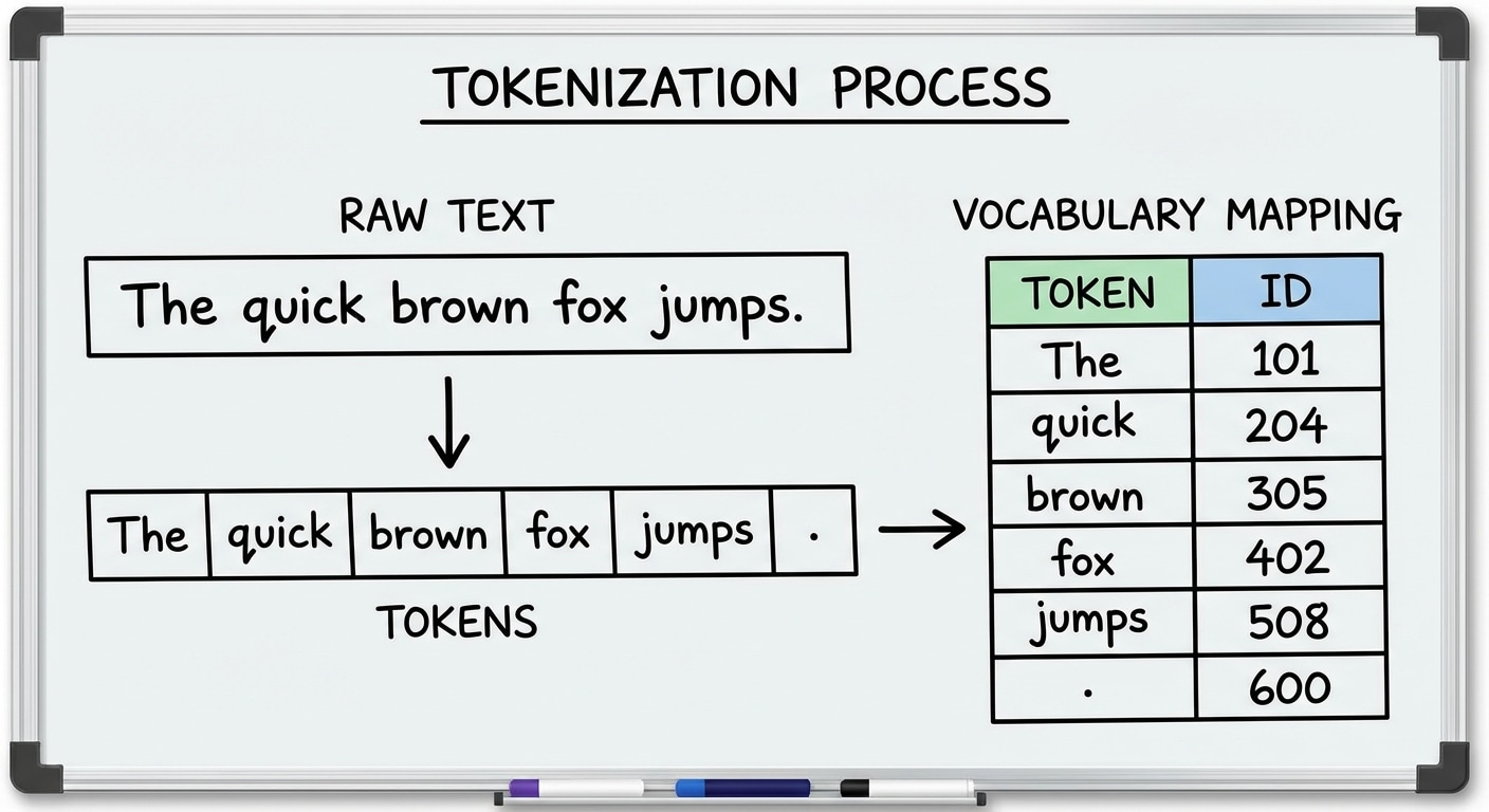
Before AI can process text, it must be split into tokens – the fundamental units the model works with. Tokenization strategy significantly impacts model performance, vocabulary size, and ability to handle rare or novel words. Getting it right matters more than many realise.
Word-level tokenization splits on whitespace, creating intuitive tokens but massive vocabularies. Unknown words become impossible to handle. Character-level uses each character as a token, handling any text but losing word-level semantics and creating very long sequences.
Subword tokenization like BPE and WordPiece offers the best of both worlds. Common words remain whole while rare words split into meaningful subwords. The vocabulary stays manageable at 32K-100K tokens while handling novel words by decomposition.
Modern tokenizers also handle special tokens for model control: beginning and end of sequence markers, padding tokens, and special separators. Understanding tokenization helps debug model behaviour – sometimes strange outputs trace back to unexpected token boundaries.
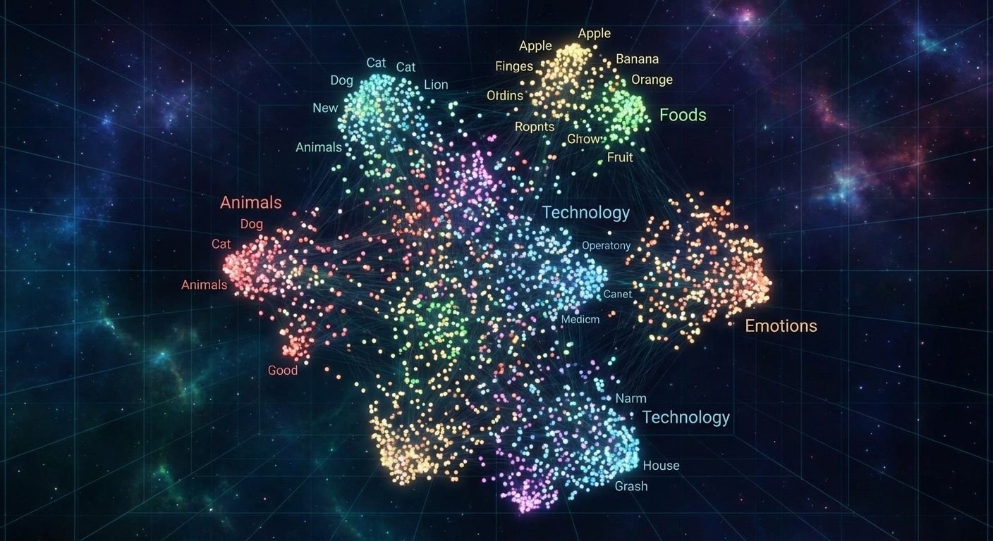
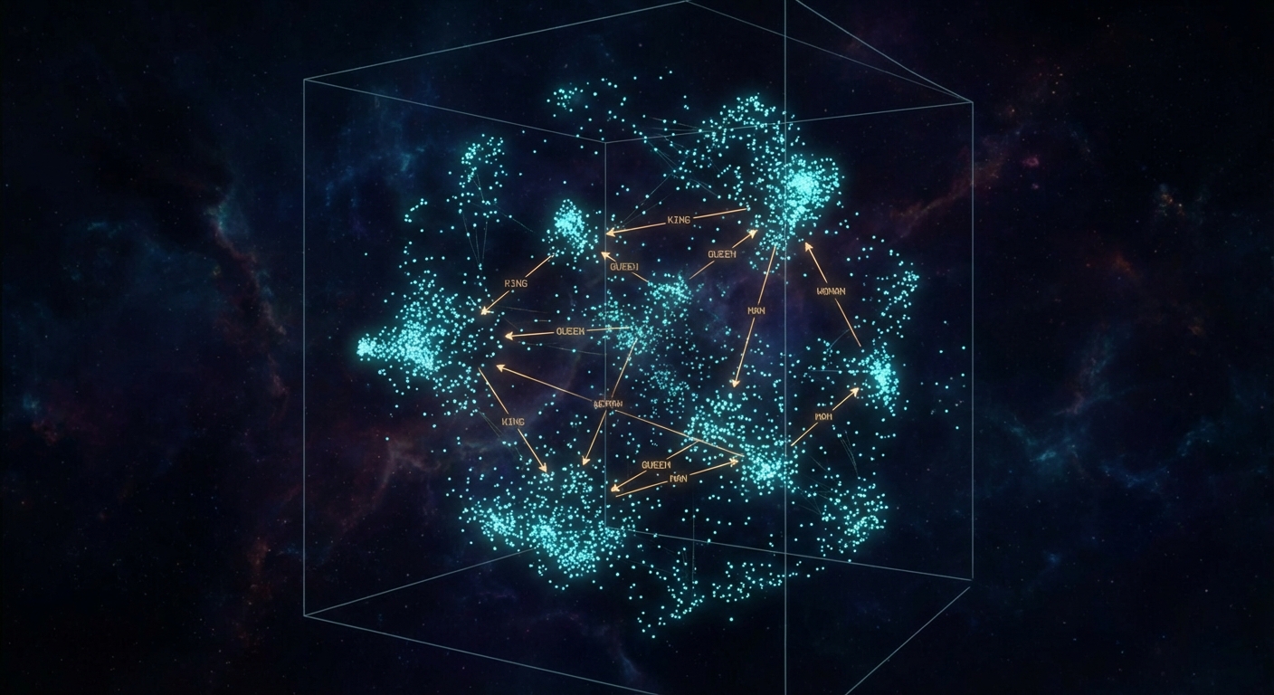
Word embeddings convert discrete tokens into dense vectors where semantic similarity corresponds to geometric proximity. This representation enables neural networks to understand that king and queen are related, or that Paris relates to France as Rome relates to Italy.
Early methods like Word2Vec learn embeddings by predicting context from words or vice versa. GloVe factors word co-occurrence matrices for global statistics. These static embeddings assign one vector per word regardless of context, missing nuances like bank meaning riverbank versus financial institution.
Contextual embeddings from BERT and GPT solved this limitation. The same word gets different representations based on surrounding context. This dynamic understanding dramatically improved performance on tasks requiring disambiguation and nuanced comprehension.
Embeddings reveal learned structure through vector arithmetic. The classic example: king minus man plus woman equals queen. These relationships emerge unsupervised from training data, demonstrating that neural networks discover meaningful semantic structure without explicit guidance.
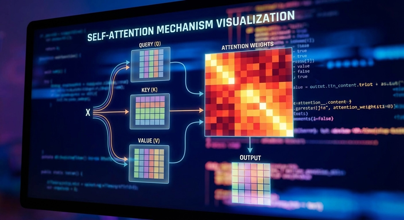
Self-attention allows each element in a sequence to attend to all other elements, capturing relationships regardless of distance. This mechanism revolutionized NLP by replacing recurrence with parallelisable attention operations that model long-range dependencies more effectively.
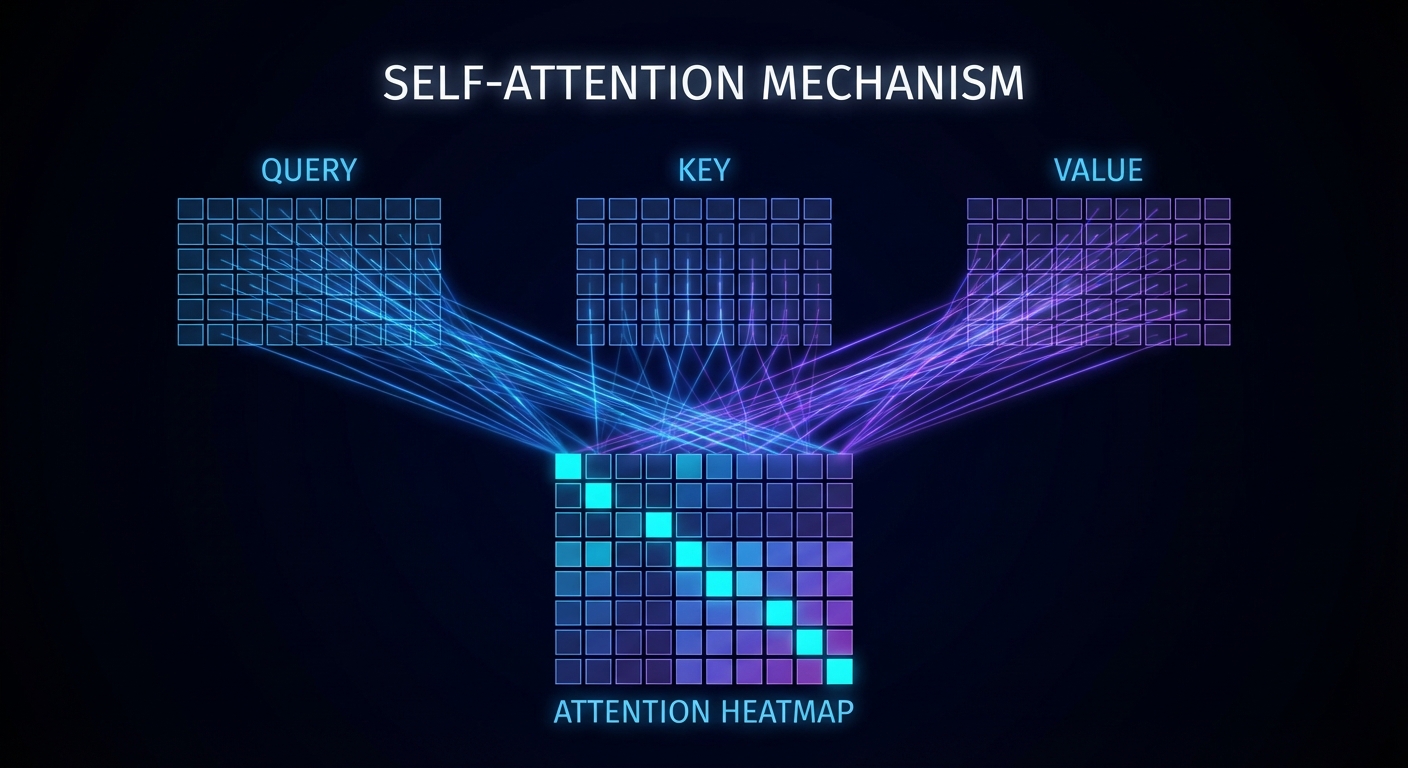
For each token, three vectors are computed: Query (what am I looking for), Key (what do I contain), and Value (what information do I provide). Attention weights come from the dot product of Query and Key, normalised by softmax. These weights determine how much each token contributes to the output.
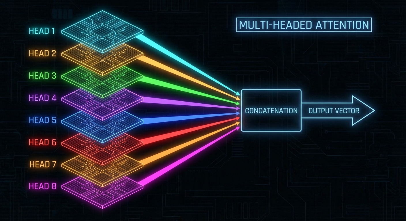
Multi-head attention runs multiple attention mechanisms in parallel, each learning to focus on different relationship types. One head might capture syntactic dependencies while another focuses on semantic similarity. Concatenating and projecting results combines these perspectives.
The attention mechanism enables remarkable capabilities in language models. A model can understand that a pronoun refers to a noun mentioned paragraphs earlier, or that a technical term definition from the context applies throughout. This contextual understanding underpins modern LLM performance.
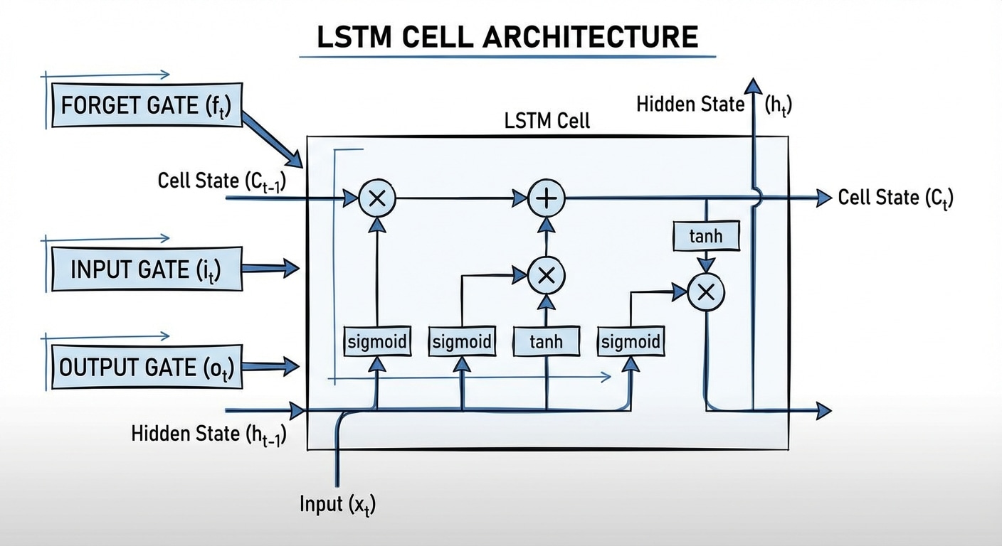
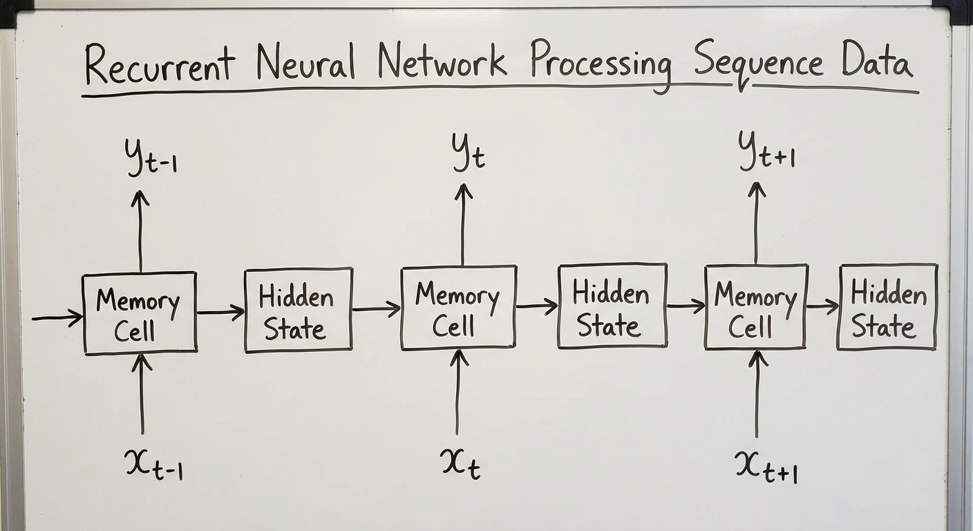
The Long Short-Term Memory (LSTM) network is a specialised kind of Recurrent Neural Network (RNN) architecture, designed specifically to solve the problem of vanishing gradients that plagues traditional RNNs when dealing with long sequences of data.
While standard RNNs struggle to retain information from many steps ago, LSTMs are engineered with a dedicated Cell State (Ct)—often called the “conveyor belt”—that runs straight through the network. This Cell State is regulated by three distinct, multiplicative gates (Forget, Input, and Output) that learn to selectively remember or forget information, allowing the network to capture and utilise long-term dependencies in sequential data like text, speech, and time series. The mathematical equations below illustrate how these gates precisely control the flow of both long-term memory (Ct) and short-term output (ht).
LSTM Cell Architecture Equations
This breakdown translates the LSTM diagram into its corresponding mathematical equations, showing exactly how the inputs (xt, ht-1, Ct-1) are processed to generate the outputs (ht, Ct).
The σ symbol represents the Sigmoid function, and W and b represent the weight matrices and bias vectors learned during training.
1. The Gates (Control)
The first step is calculating the three gates, each using the current input (xt) and the previous hidden state (ht-1) and applying a sigmoid function (σ):
A. Forget Gate (ft):
ft = σ(Wf · [ht-1, xt] + bf)
Purpose: Decides which information to forget from the old cell state (Ct-1).
B. Input Gate (it):
it = σ(Wi · [ht-1, xt] + bi)
Purpose: Decides which values to update in the cell state.
C. Candidate Cell State (ᶜt):
ᶜt = tanh(WC · [ht-1, xt] + bC)
Purpose: Creates a vector of potential new values that could be added to the cell state.
2. Cell State Update (The Memory)
The Cell State (Ct) is the core memory of the LSTM, updated by combining the old memory and the new candidate memory:
Ct = ft ∗ Ct-1 + it ∗ ᶜt
The term ft * Ct-1 implements the forgetting mechanism: the old memory Ct-1 is scaled down by the Forget Gate ft.
The term it * ᶜt implements the input mechanism: the new candidate information ᶜt is scaled by the Input Gate it.
These two parts are then added to create the new long-term memory, Ct.
3. Hidden State Output (The Prediction)
The Hidden State (ht) is the final output of the cell at this time step. It is based on the new Cell State, filtered by the Output Gate:
A. Output Gate (ot):
ot = σ(Wo · [ht-1, xt] + bo)
Purpose: Decides which parts of the (squashed) Cell State will be exposed as the Hidden State.
B. Final Hidden State (ht):
ht = ot ∗ tanh(Ct)
The new Cell State Ct is passed through tanh to bound the values between -1 and 1.
The result is then element-wise multiplied by the Output Gate ot to produce the final short-term memory and output vector, ht.
Conclusion: The Importance of Selective Memory
The LSTM architecture, as described by these equations, fundamentally improved the capability of recurrent neural networks to model complex dependencies over long sequences. By using three learned, multiplicative gates to regulate the flow into and out of the Cell State, the LSTM is able to maintain a stable, uncorrupted memory path, overcoming the practical limitations of standard RNNs.
This innovation has made LSTMs essential tools in areas requiring deep contextual understanding, leading to breakthroughs in speech recognition, machine translation, and text generation, before the wider adoption of the Transformer architecture.
Next Steps
Interested in a simpler alternative? Check out the GRU (Gated Recurrent Unit), which combines the forget and input gates into a single update gate—achieving similar performance with fewer parameters. For cutting-edge sequence modeling, explore how Transformers use attention mechanisms to process entire sequences in parallel, bypassing recurrence altogether.
RNNs were designed for sequential data – text, time series, audio, and video. Unlike feedforward networks that process fixed-size inputs, RNNs maintain a hidden state that acts as memory, allowing information to persist across the sequence and enabling context-aware processing.
At each timestep, the hidden state combines the previous state with new input through learned transformations. This recurrence creates a computational graph that unfolds through time, theoretically allowing information from early inputs to influence later processing indefinitely.
In practice, vanilla RNNs struggle with long sequences due to vanishing gradients. When backpropagating through many timesteps, gradients shrink exponentially, causing the network to forget early information. Exploding gradients present the opposite problem, causing training instability.
While largely superseded by Transformers for most applications, understanding RNNs remains valuable. They introduced key concepts like sequence modeling and temporal dependencies. LSTM and GRU variants solved the gradient problems, and some real-time applications still benefit from RNNs streaming nature.
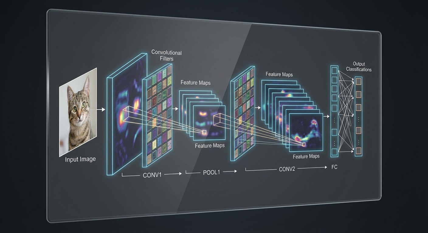
CNNs revolutionized computer vision by mimicking how the visual cortex processes images. Small learnable filters slide across the image detecting features, with early layers finding edges and later layers identifying complex objects. This hierarchical feature learning made accurate image recognition possible.
Key components include convolutional layers where filters detect local patterns, pooling layers that reduce spatial dimensions while preserving important features, and fully connected layers that combine features for final classification. The architecture dramatically reduces parameters through weight sharing.
CNNs achieve translation invariance – they detect features regardless of position in the image. A cat in the corner is recognised the same as one in the centre. This property emerges naturally from the sliding filter approach and makes CNNs robust to object placement.
Famous architectures include LeNet (1998), AlexNet (2012) which sparked the deep learning revolution, VGG demonstrating depth matters, ResNet enabling 100+ layer networks with skip connections, and modern EfficientNets balancing accuracy and efficiency. Each advanced our understanding of what makes CNNs effective.
Without activation functions, neural networks would be limited to linear transformations no matter how many layers they have. Activations introduce non-linearity, enabling networks to learn complex patterns like image recognition and language understanding that linear models cannot capture.
ReLU (Rectified Linear Unit) outputs max(0,x) – simple, fast, and surprisingly effective. It has become the default for hidden layers. Sigmoid squashes output to 0-1, useful for binary classification but prone to vanishing gradients. Tanh outputs -1 to 1, zero-centred which sometimes helps training.
For output layers, the choice depends on your task. Sigmoid for binary classification, softmax for multi-class (outputs sum to 1 as probabilities), and linear for regression. Modern variants like GELU and Swish offer slight improvements in specific contexts.
Understanding activations helps diagnose training issues. Dead ReLU neurons that never activate, saturated sigmoids causing vanishing gradients, and numerical instability all relate to activation choice. Experimentation within established guidelines usually yields good results.
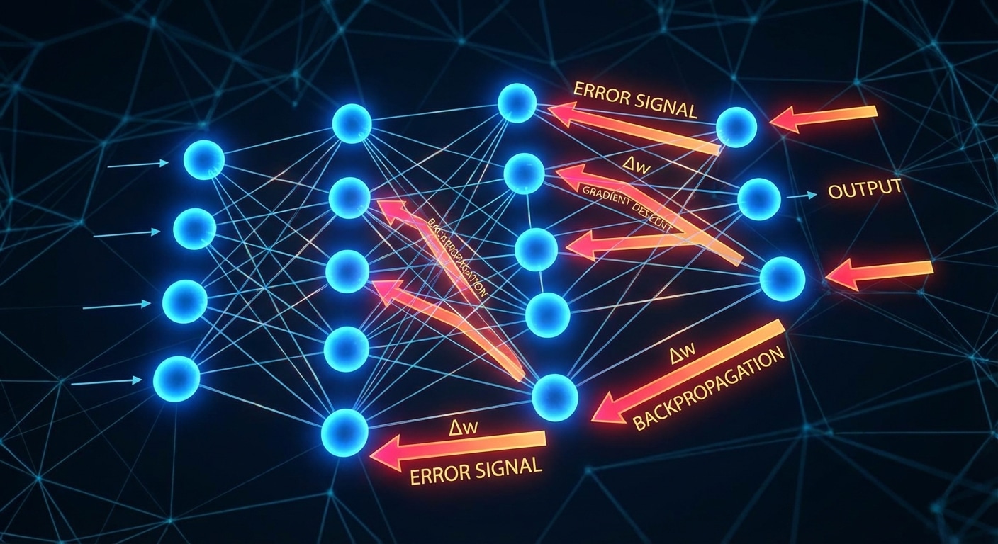
Backpropagation is the algorithm that makes deep learning possible. It efficiently computes how much each weight in a neural network contributed to the prediction error, enabling targeted updates that improve performance. Without backprop, training deep networks would be computationally infeasible.
The algorithm applies the calculus chain rule to propagate error gradients backward through the network. Starting from the output layer, it calculates local gradients then multiplies by downstream gradients to determine each weights contribution to the loss. This recursive computation handles arbitrarily deep networks.
The beauty of backpropagation lies in its efficiency. It computes all gradients in a single backward pass through the network, achieving O(n) complexity. Computing each gradient independently would require O(n squared) forward passes, making training prohibitively slow for modern architectures.
Understanding backprop illuminates common training issues. Vanishing gradients occur when gradients shrink exponentially through layers. Exploding gradients cause instability. Techniques like gradient clipping, proper initialisation, and batch normalisation address these issues while preserving backprops fundamental efficiency.
Deep learning derives its name from having many layers, but depth accomplishes more than just size. Each layer builds increasingly abstract representations, transforming raw inputs into meaningful features. This hierarchical learning mirrors how the visual cortex processes information from simple edges to complex objects.
In image recognition, early layers detect edges and simple patterns. Middle layers combine these into textures and shapes. Deeper layers recognise parts like eyes or wheels. Final layers identify complete objects and scenes. This progression from concrete to abstract happens automatically through training.
Deeper networks can represent more complex functions with fewer parameters than shallow networks. However, training deep networks historically faced the vanishing gradient problem where gradients became infinitesimally small in early layers. Innovations like ReLU activation and residual connections solved this, enabling networks with hundreds of layers.
Understanding layer-wise abstraction helps in architecture design and debugging. Visualising intermediate activations reveals what each layer learns. Transfer learning exploits this by reusing early general-purpose layers while fine-tuning later task-specific ones.
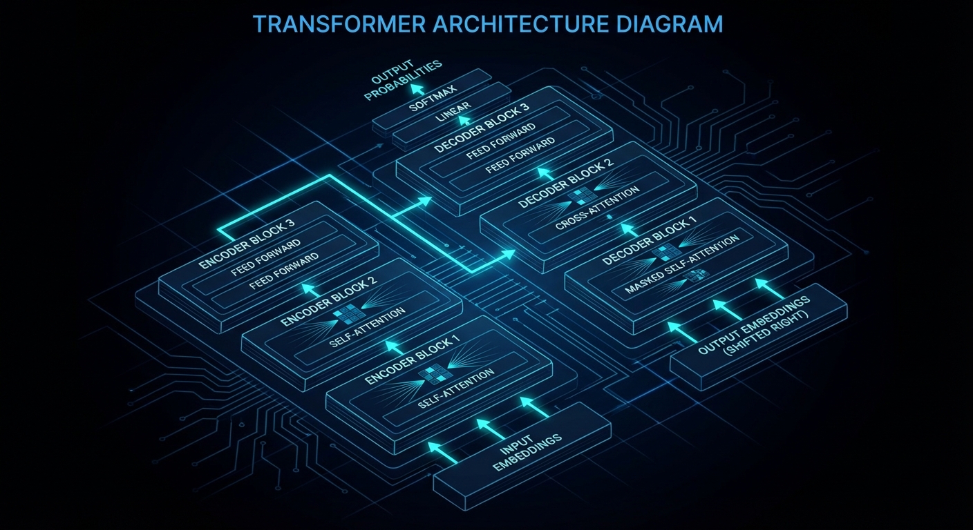
If you have used ChatGPT, Google Translate, Stable Diffusion, or Whisper, you have used a transformer. The word keeps appearing everywhere, yet most explanations either wave their hands at “attention” and call it magic, or dump the full paper on you without mercy. This article is neither. We are going to open the thing up, trace data as it flows from raw text to a probability distribution over the next word, and understand every matrix multiplication along the way. By the end, the architecture will not feel like a black box; it will feel like a very elegant piece of engineering that you could, in principle, rebuild yourself.
Data flows left-to-right through stacked attention and feed-forward blocks. Every step is a matrix multiplication.
Where Transformers Came From (and Why Everything Before Them Was Painful)
Before 2017, the dominant approach to sequence modelling was the recurrent neural network, or RNN, and its variants: LSTMs and GRUs. The core idea was sensible enough: process tokens one at a time, left to right, carrying a hidden state forward like a running summary of what you have seen so far. The problem was that this sequential processing was fundamentally slow, because you could not parallelise across time steps. Worse, gradients had to flow backwards through every single time step during training, which caused the infamous vanishing gradient problem: information from early in a long sequence would be diluted almost to nothing by the time it reached the end.
In June 2017, eight researchers at Google published a paper titled “Attention Is All You Need”. The title was a provocation. They were arguing that the recurrent structure was not just slow but unnecessary, that a mechanism called attention could do everything a recurrent network could do, better and faster, without any sequential processing at all.
They were right. Within a few years, transformers had conquered not just natural language processing but computer vision, speech recognition, protein structure prediction, and more. GPT-3, released in 2020, has 175 billion parameters organised into just under 28,000 distinct matrices that fall into eight categories. This article will walk through all of them.
The High-Level Loop: Predict, Sample, Repeat
Before diving into the internals, it helps to understand what the whole machine is actually trying to do. The variant we will focus on, the decoder-only transformer that underlies GPT, is a next-token predictor. You feed it a sequence of text, and it outputs a probability distribution over what token is most likely to come next.
Generating a longer passage is then just a loop:
# Pseudocode for autoregressive generation
context = "Once upon a time"

for step in range(max_tokens):
    # Run the full transformer forward pass
    logits = transformer.forward(context)           # shape: [vocab_size]
    probs  = softmax(logits / temperature)          # probability distribution
    next_token = sample(probs)                      # pick one token stochastically
    context = context + next_token                  # append and repeat
    if next_token == END_OF_SEQUENCE:
        break
That loop is, at a high level, what you are watching when ChatGPT produces one word at a time. The transformer is not generating the whole sentence at once and then typing it out; it is literally running this predict-sample-append cycle for every single token. The “intelligence” is entirely in what the forward pass computes.
Step 1: Tokenisation
Text is not numbers. The first job is to convert a raw string into a sequence of integers that the model can work with. This is tokenisation. Modern LLMs almost never tokenise on full words; they use a subword algorithm called Byte Pair Encoding (BPE), which learns a vocabulary of common character sequences from the training corpus.
GPT-3 uses a vocabulary of 50,257 tokens. The word “unbelievable” might be split into [“un”, “believ”, “able”], while a common word like “the” gets a single token. Punctuation, spaces, and even code syntax all have their own tokens. The key point is that every possible input string can be faithfully represented as a sequence of tokens drawn from this fixed vocabulary.
import tiktoken  # OpenAI's tokeniser library

enc = tiktoken.encoding_for_model("gpt-3.5-turbo")

text = "The Transformer architecture is surprisingly elegant."
tokens = enc.encode(text)
print(tokens)
# [464, 3602, 16354, 10478, 318, 7051, 33687, 13]

# Each integer maps to a token string:
for tok in tokens:
    print(repr(enc.decode([tok])))
Those integers are what actually enter the network. Everything from here on is floating-point arithmetic on sequences of integers.
Step 2: The Embedding Matrix — Turning Integers into Geometry
An integer like 464 is useless for a neural network. We need to turn it into a vector of continuous numbers that can participate in matrix multiplications. This is the job of the embedding matrix, denoted W_E.
W_E has one column per vocabulary token and one row per embedding dimension. For GPT-3, that is 50,257 columns × 12,288 rows, giving roughly 617 million parameters just for this one matrix. Looking up the embedding for a token is literally just selecting the corresponding column.
Words live as points in 12,288-dimensional space. Directions carry semantic meaning: gender, plurality, syntax.
The remarkable thing that emerges during training is that directions in this 12,288-dimensional space acquire semantic meaning. The classic demonstration is the gender direction: the vector from “man” to “woman” is approximately the same as the vector from “king” to “queen”. Plurality, verb tense, country-to-capital relationships, all of these end up encoded as consistent geometric directions. This is not something the architects programmed in; it emerged purely from gradient descent on a next-token prediction objective.
This property was first described in the Word2Vec paper by Mikolov et al. in 2013, which demonstrated that a simple shallow neural network trained on next-word prediction would spontaneously develop embeddings with these arithmetic properties. The transformer embedding space is a much higher-dimensional descendant of the same idea.
import numpy as np

# Conceptual example: arithmetic in embedding space
# (using a pre-trained model's actual embeddings)

embed = model.get_embedding  # function: word -> vector

king   = embed("king")
queen  = embed("queen")
man    = embed("man")
woman  = embed("woman")

# The gender direction
gender_direction = woman - man

# Does king + gender_direction ≈ queen?
predicted_queen = king + gender_direction
cosine_sim = np.dot(predicted_queen, queen) / (
    np.linalg.norm(predicted_queen) * np.linalg.norm(queen)
)
print(f"Cosine similarity: {cosine_sim:.3f}")  # ~0.85 in practice
You should think of dot products as the workhorse similarity measure here. The dot product of two vectors is positive when they point in similar directions, zero when perpendicular, and negative when opposing. This geometric interpretation will be critical when we get to attention.
Step 3: Positional Encoding — Teaching the Model Where Things Are
Here is a problem: the embedding of “dog” is identical whether it appears first or last in the sentence. The transformer processes all tokens in parallel, which means it has no inherent sense of order. We have to give it one explicitly.
The original 2017 paper used a fixed sinusoidal encoding: for each position p and each dimension i of the embedding, you add a value derived from sin or cos at a frequency that scales with i. The frequencies were chosen so that each position produces a unique pattern, and so that the difference between adjacent positions is consistent regardless of absolute position. Modern models like GPT-3 use learned positional embeddings instead, treating position as just another lookup table. More recent work uses Rotary Position Embeddings (RoPE, Su et al. 2021) or ALiBi (Press et al. 2022), which encode relative rather than absolute position and generalise better to sequences longer than those seen during training.
import torch
import torch.nn as nn

class TransformerEmbedding(nn.Module):
    def __init__(self, vocab_size, embed_dim, max_seq_len):
        super().__init__()
        # Token embeddings: one vector per vocabulary item
        self.token_embed    = nn.Embedding(vocab_size, embed_dim)
        # Positional embeddings: one vector per possible position
        self.position_embed = nn.Embedding(max_seq_len, embed_dim)

    def forward(self, token_ids):
        # token_ids: shape [batch_size, seq_len]
        seq_len   = token_ids.size(1)
        positions = torch.arange(seq_len, device=token_ids.device)

        tok_vecs = self.token_embed(token_ids)       # [batch, seq, embed_dim]
        pos_vecs = self.position_embed(positions)    # [seq, embed_dim]

        # Simply add the two: each vector now encodes both identity and position
        return tok_vecs + pos_vecs
The key insight is that we simply add the positional vector to the token vector. Both live in the same 12,288-dimensional space, so the addition is well-defined. The resulting vectors now simultaneously encode what the token is and where it sits in the sequence.
Step 4: Self-Attention — The Heart of the Transformer
We now have a sequence of vectors, one per token, each encoding identity and position. The problem is that these vectors are still context-free. The embedding of “mole” is identical whether it appears in “one mole of carbon dioxide”, “take a biopsy of the mole”, or “American shrew mole”. Self-attention is the mechanism that fixes this by allowing every token to gather information from every other token in the sequence.
Before the 2017 paper, attention mechanisms already existed as an add-on to RNNs, used to help encoder-decoder models for translation decide which input tokens to focus on when producing each output token. Bahdanau et al. demonstrated this in 2014. What Vaswani et al. did was remove the RNN entirely and let attention carry the full weight of the architecture. “All You Need”, as it says on the tin.
Each token asks a query, every token broadcasts a key, and dot products between them produce the attention pattern.
The mechanism works through three learned matrices: the query matrix W_Q, the key matrix W_K, and the value matrix W_V. Here is what each one does conceptually:
Query (W_Q): Each token uses this matrix to produce a “question” vector. For example, a noun might produce a query that encodes “looking for adjectives that describe me”.
Key (W_K): Each token uses this matrix to produce an “answer” vector. An adjective might produce a key that encodes “I am an adjective, and I modify things”.
Value (W_V): Each token uses this matrix to produce the actual information it wants to share. If an adjective is deemed relevant to a noun, the value vector specifies what should be added to the noun’s embedding.
For a sequence of n tokens with embeddings E (shape n × d_model), you compute:
import torch
import torch.nn.functional as F
import math

def single_head_attention(E, W_Q, W_K, W_V, mask=None):
    """
    E:    [n, d_model]  - token embeddings
    W_Q:  [d_model, d_k]
    W_K:  [d_model, d_k]
    W_V:  [d_model, d_v]
    """
    d_k = W_Q.shape[1]

    # Step 1: Compute queries, keys, and values
    Q = E @ W_Q   # [n, d_k]  - each token asks a question
    K = E @ W_K   # [n, d_k]  - each token broadcasts an answer
    V = E @ W_V   # [n, d_v]  - each token prepares information to share

    # Step 2: Compute attention scores via dot products
    # scores[i][j] = how relevant is token j to updating token i
    scores = Q @ K.T / math.sqrt(d_k)   # [n, n]

    # Step 3: Apply causal mask (prevent future tokens influencing past)
    if mask is not None:
        scores = scores.masked_fill(mask == 0, float('-inf'))

    # Step 4: Softmax over each row -> probability distribution per query
    weights = F.softmax(scores, dim=-1)  # [n, n]

    # Step 5: Weighted sum of values
    output = weights @ V                 # [n, d_v]
    return output, weights
The division by √d_k is a small but important numerical stability trick. Without it, when the key-query dimension is large, the dot products grow very large in magnitude, pushing the softmax into regions where its gradient approaches zero and training stalls.
“We suspect that for large values of d_k, the dot products grow large in magnitude, pushing the softmax function into regions where it has extremely small gradients. To counteract this effect, we scale the dot products by 1/√d_k.” — Vaswani et al., “Attention Is All You Need”, arXiv:1706.03762
The Attention Pattern and Masking
The matrix of softmax-normalised dot products is called the attention pattern. It is an n×n grid where entry (i, j) represents how much token i attends to token j when refining its embedding. In a well-trained model, the noun “creature” would have high attention weights for preceding adjectives “fluffy” and “blue”, and low weights for articles like “the”.
For decoder-only (autoregressive) models like GPT, there is a hard constraint: token i must not be able to attend to token j if j > i. If it could, the model would be cheating during training, peeking at the answer. This is enforced by causal masking: before applying softmax, set all scores where j > i to −∞. After softmax, those positions become exactly 0.
def causal_mask(n):
    """Upper triangular mask: 1 = allowed, 0 = masked out."""
    return torch.tril(torch.ones(n, n))

# Visualising a 5-token causal mask:
# Token:  0  1  2  3  4
# t=0  [  1  0  0  0  0 ]  # can only see itself
# t=1  [  1  1  0  0  0 ]  # can see token 0 and itself
# t=2  [  1  1  1  0  0 ]
# t=3  [  1  1  1  1  0 ]
# t=4  [  1  1  1  1  1 ]  # can see the full context so far
Encoder-only models like BERT do not apply causal masking: every token can attend to every other token in both directions simultaneously. This bidirectional attention is why BERT excels at tasks like classification and question answering, where you have the full input available, but it cannot generate text autoregressively the way GPT can.
There is also a practical consequence of attention’s O(n²) memory complexity: the attention pattern grows with the square of the context length. A 4,096-token context needs an attention pattern of 4,096 × 4,096 = 16.7 million values per head per layer. This is exactly why extending context windows is non-trivial, and why techniques like FlashAttention exist.
FlashAttention does not approximate or skip any computation; it produces mathematically identical results to standard attention. The trick is to recompute attention scores in tiles that fit in fast SRAM, rather than materialising the full n×n matrix in slow HBM. On modern GPUs this produces a 2–4× speedup and reduces memory from O(n²) to O(n), making 100K+ token contexts feasible on a single device.
The Attention Mechanism: A Deeper Look
The Q/K/V description above gives you the mechanics. But if you stop there, you will build correct code that you do not truly understand. Let us go deeper, because the attention mechanism has a rich internal structure that becomes important when you need to debug it, scale it, or reason about what a model has learnt.
The Residual Stream View
The most clarifying way to think about a transformer — and one that Anthropic’s interpretability team uses extensively — is not as a pipeline that transforms embeddings, but as a sequence of additions to a shared residual stream. Every token has one vector in this stream, initialised by the embedding lookup. Every sub-block, whether attention head or FFN layer, reads from this stream and writes an additive update back to it. Nothing is overwritten; everything is accumulated.
# The residual stream perspective
# x[t] is the state vector for token t after layer L

# At layer 0: just the embedding + positional encoding
x = embed(token) + pos_embed(position)   # shape: [d_model]

# Each attention head reads x, computes a delta, adds it
for head in attention_heads:
    delta = head.compute_update(x_all_tokens)
    x = x + delta    # <-- additive write to residual stream

# Each FFN layer also reads x, adds its delta
delta_ffn = ffn.forward(x)
x = x + delta_ffn   # <-- another additive write

# By the final layer, x encodes everything the network has
# decided is relevant about this token in this context
This view matters because it means every layer's output is implicitly competing to write useful information into a shared finite-dimensional space. Early layers tend to handle syntax and local structure; later layers handle semantics, coreference, and world knowledge. The residual connection ensures that if a layer has nothing useful to contribute, it can learn to output near-zero updates and leave the stream unchanged, rather than corrupting earlier representations. This is why very deep transformers train at all without layer-by-layer degradation. The idea connects directly to the residual networks (ResNets) that He et al. introduced for computer vision in 2015, and which the transformer architects borrowed wholesale.
Within a single attention head, there are actually two conceptually distinct computations happening, which Anthropic's framework calls the QK circuit and the OV circuit. Understanding them separately makes the head much easier to reason about.
The QK circuit determines where information flows. It computes the attention pattern: which tokens attend to which other tokens. Mathematically, this is determined entirely by the product W_Q^T W_K. You can think of it as a bilinear form: for two token embeddings x and y, the attention score is x^T (W_Q^T W_K) y. The QK circuit therefore describes a learned notion of "relevance" between pairs of tokens in the residual stream.
The OV circuit determines what information is copied. Given that the attention pattern says "attend here", the OV circuit specifies what gets written into the residual stream as a result. This is determined by the product W_V W_O (value matrix times output projection matrix). The OV circuit is a linear map from the source token's residual stream to an update added to the destination token's residual stream.
import torch

def analyse_attention_head(W_Q, W_K, W_V, W_O):
    """
    Decompose an attention head into its QK and OV circuits.

    W_Q: [d_model, d_k]   - query projection
    W_K: [d_model, d_k]   - key projection
    W_V: [d_model, d_v]   - value projection (value-down in 3B1B's framing)
    W_O: [d_v, d_model]   - output projection (value-up)
    """

    # The QK circuit: a d_model x d_model matrix representing
    # "how much does token x's embedding cause it to attend to token y's embedding"
    QK_circuit = W_Q @ W_K.T    # [d_model, d_model]

    # The OV circuit: a d_model x d_model matrix representing
    # "if token x attends to token y, what gets added to token x's residual stream"
    OV_circuit = W_V @ W_O      # [d_model, d_model]

    # Eigenvalues of OV tell you what the head "copies":
    # large positive eigenvalues = the head reinforces certain directions
    # near-zero eigenvalues = the head ignores those directions
    eigenvalues = torch.linalg.eigvals(OV_circuit).real
    print(f"OV circuit rank estimate: {(eigenvalues.abs() > 0.01).sum().item()}")

    return QK_circuit, OV_circuit
This decomposition is not just theoretical tidiness. It has a practical consequence: if you want to understand what a specific attention head has learnt, you can compute its OV circuit and look for interpretable structure. Anthropic's circuit analysis found heads where the OV circuit is essentially a "copy" operation, moving the source token's own embedding directly into the destination. These are called copy heads, and they appear consistently across different models.
Induction Heads: A Concrete Example of What Heads Actually Learn
Here is the most well-studied concrete example of an attention circuit in real models. Suppose your input contains the sequence [A][B] ... [A], where A and B are tokens and there is some distance between the first [A][B] pair and the second [A]. After seeing the second [A], a well-trained model should assign high probability to [B] as the next token, because it saw that pattern before.
This in-context pattern copying is carried out by a two-head circuit known as an induction circuit, and it appears in essentially every transformer large enough to contain it. The circuit consists of:
A previous-token head in an early layer. This head has a simple QK circuit that makes every token attend strongly to the token immediately before it. Its OV circuit copies the previous token's embedding into the current token's residual stream.
An induction head in a later layer. This head uses a QK circuit that makes a token attend to the previous occurrence of whatever token currently precedes it in the stream (which, after the previous-token head ran, is encoded in the current token's representation).
# Conceptual trace of an induction circuit for sequence [A][B]...[A][?]
# Positions:                                              0   1       k  k+1

# After previous-token head (layer 1):
# residual[k] now contains information about token at position k-1
# i.e., residual at position k encodes "I am A, and the token before me is [A-1]"
# (where [A-1] is whatever preceded the first A)

# After induction head (layer 2):
# Token at position k+1 asks: "find me the token that follows
#   whatever token currently precedes me"
# The previous-token head already wrote "token k-1" into residual[k]
# So the induction head attends to position 1 (the first [B]),
#   because position 1 follows the previous occurrence of what precedes k
# OV circuit copies B's embedding -> high logit for B as next token

# Net result: the model predicts [B] after the second [A],
# using only information available in context (no memorisation required)
Why does this matter to you as an engineer? Because induction circuits are the mechanical basis of in-context learning, the GPT behaviour where you give a few examples in the prompt and the model generalises the pattern to new inputs. Understanding this circuit is the first step towards understanding when and why few-shot prompting works, and when it does not.
What Different Heads Specialise In
Research on attention head specialisation across models has found several recurring functional types, described in Voita et al.'s 2019 analysis of BERT and in subsequent mechanistic interpretability work:
Positional heads: attend to fixed relative positions (e.g., always the previous token, always the next token). These handle local syntactic structure.
Syntactic heads: implement specific grammatical relations — subject-verb, noun-adjective, pronoun-antecedent. These have been probed extensively in BERT-style models.
Copy heads / duplicate token heads: move information about the current token's identity to future positions, enabling long-range pattern matching.
Induction heads: described above, the in-context pattern-matching circuit.
Attention sinks: every sufficiently large transformer appears to develop heads that attend heavily to the first token in the sequence regardless of content. Mistral's paper on Sliding Window Attention noted this; it seems to serve as a no-op or "null" option when no other token is strongly relevant.
Not every head has a clean human-interpretable function. Many heads appear to operate through superposition: the same neurons and weights simultaneously represent multiple features in different contexts, making clean labels impossible. This is an active area of research, and the honest answer is that most heads in most models remain poorly understood.
Why Dot-Product Attention Works Geometrically
The dot product appears throughout attention, and it helps to have a clear geometric intuition for why it is the right operation. Given two vectors u and v, their dot product u·v = |u||v|cos(θ), where θ is the angle between them. This means:
If u and v point in the same direction, the dot product is large and positive.
If they are perpendicular, the dot product is exactly zero.
If they point in opposite directions, the dot product is large and negative.
In the attention mechanism, the query vector for token i and the key vector for token j live in the same d_k-dimensional space. A large positive dot product means the query and key "point in the same direction", which after training corresponds to "this key is answering the question the query is asking". The model learns W_Q and W_K such that relevant query-key pairs end up geometrically aligned, and irrelevant pairs end up perpendicular or opposed.
import torch
import torch.nn.functional as F

def attention_geometry_demo():
    d_k = 128

    # Suppose we have a query for "noun looking for adjective"
    # and two keys: one for "adjective" and one for "verb"
    query_noun       = torch.randn(d_k)
    key_adjective    = torch.randn(d_k)
    key_verb         = torch.randn(d_k)

    # After training, we would hope that:
    # query_noun . key_adjective >> query_noun . key_verb

    # Before training (random initialisation), they are roughly equal:
    score_adj  = torch.dot(query_noun, key_adjective) / (d_k ** 0.5)
    score_verb = torch.dot(query_noun, key_verb)      / (d_k ** 0.5)
    print(f"Random init — adj: {score_adj:.2f}, verb: {score_verb:.2f}")

    # After training the model has learnt W_Q and W_K such that
    # the projected query and key vectors for relevant pairs align:
    # (W_Q @ embed_noun) . (W_K @ embed_adj) >> (W_Q @ embed_noun) . (W_K @ embed_verb)
    # The softmax then converts these scores to attention weights:
    scores  = torch.tensor([2.5, -1.2, 0.3, -0.8])  # example scores
    weights = F.softmax(scores, dim=0)
    print(f"Attention weights: {weights}")
    # The first token (adjective) dominates the distribution
Attention Across Layers: Early vs Late
Stacking 96 attention layers is not just "more of the same". Different layers handle qualitatively different kinds of context integration, and this has been confirmed empirically through probing studies and ablation experiments.
Early layers (1–20 in GPT-3): attention patterns tend to be local and syntactic. Heads attend to adjacent tokens, to punctuation delimiters, to syntactic heads of phrases. The residual stream at this point is being transformed from "token at position p" into something more like "syntactic unit of type X at position p".
Middle layers (20–60): attention patterns become more global and semantic. Coreference resolution (connecting a pronoun to its antecedent) happens here. Induction-style pattern matching operates here. The representations start to encode word sense and shallow world knowledge.
Late layers (60–96): attention becomes task-specific. Heads in these layers appear to be doing the final aggregation that feeds into the next-token prediction. Probing classifiers trained on late-layer representations can predict the correct next token much better than those trained on early-layer representations. This is where the model is "deciding what to say".
This layered specialisation is part of why you can fine-tune just the last few layers of a pre-trained transformer for a new task and get surprisingly good results: the early layers are doing general linguistic processing that transfers cleanly, and only the final prediction-relevant layers need updating for the new domain. This intuition is formalised in the transfer learning literature, particularly in the BERT fine-tuning papers by Devlin et al., which showed that even adding a single linear layer on top of BERT's final representations was sufficient for many classification tasks.
The Attention Pattern Is Not "Explanation"
There is a widespread and wrong interpretation of attention weights as explanations: "the model attended to token X, therefore token X caused the prediction". This does not follow. Jain and Wallace (2019) showed that attention weights often do not correlate with feature importance as measured by gradient-based methods, and that you can substitute in near-uniform attention weights in many cases and get identical outputs. The attention pattern tells you where information was routed; it does not tell you what that information was, how it was transformed by the OV circuit, or whether it was the decisive factor in the output.
The right way to think about attention weights is as a routing mechanism, not an explanation. You need the full QK circuit plus the OV circuit to understand what a head is doing, and even then, the interaction between 96 heads across 96 layers is not something you can summarise in a heatmap.
Step 5: Multi-Headed Attention — Running Many Conversations in Parallel
A single attention head can capture one type of relationship between tokens: adjectives modifying nouns, or pronouns resolving their referents, or a verb attending to its subject. Real language has many such relationships operating simultaneously. Multi-headed attention runs H separate attention heads in parallel, each with its own W_Q, W_K, and W_V matrices, producing H independent attention patterns and H independent sets of updates.
GPT-3 runs 96 attention heads per layer. Each head can specialise in a different type of contextual relationship.
import torch
import torch.nn as nn
import torch.nn.functional as F
import math

class MultiHeadAttention(nn.Module):
    def __init__(self, d_model, num_heads):
        super().__init__()
        assert d_model % num_heads == 0
        self.num_heads = num_heads
        self.d_k = d_model // num_heads  # dimension per head

        # All heads' Q, K, V projections packed into single matrices
        self.W_Q = nn.Linear(d_model, d_model, bias=False)
        self.W_K = nn.Linear(d_model, d_model, bias=False)
        self.W_V = nn.Linear(d_model, d_model, bias=False)
        # Output projection (the "value up" matrix in 3B1B's framing)
        self.W_O = nn.Linear(d_model, d_model, bias=False)

    def forward(self, x, mask=None):
        B, n, d = x.shape   # batch, sequence length, model dim

        # Project and split into H heads
        Q = self.W_Q(x).view(B, n, self.num_heads, self.d_k).transpose(1, 2)
        K = self.W_K(x).view(B, n, self.num_heads, self.d_k).transpose(1, 2)
        V = self.W_V(x).view(B, n, self.num_heads, self.d_k).transpose(1, 2)
        # Shape: [B, num_heads, n, d_k]

        # Scaled dot-product attention for all heads simultaneously
        scores = Q @ K.transpose(-2, -1) / math.sqrt(self.d_k)
        if mask is not None:
            scores = scores.masked_fill(mask == 0, float('-inf'))
        weights = F.softmax(scores, dim=-1)

        # Weighted sum of values
        attended = weights @ V         # [B, num_heads, n, d_k]

        # Concatenate heads and project back to d_model
        attended = attended.transpose(1, 2).contiguous().view(B, n, d)
        return self.W_O(attended)      # [B, n, d_model]
In GPT-3 each layer has 96 heads. The embedding dimension is 12,288, so each head works in a 128-dimensional subspace (12,288 / 96 = 128). The key and query matrices are each 12,288 × 128; four such matrices per head × 96 heads × 96 layers yields just under 58 billion of the model's 175 billion parameters. Attention gets all the attention, but it is only about a third of the total parameter budget.
Step 6: The Feed-Forward Block — Where the Facts Live
After each multi-headed attention block, the token embeddings pass through a feed-forward network (FFN), sometimes called a multi-layer perceptron (MLP). Unlike attention, the FFN does not allow tokens to communicate with each other; it processes each position independently and identically.
class FeedForward(nn.Module):
    def __init__(self, d_model, d_ff):
        super().__init__()
        # d_ff is typically 4 * d_model
        # For GPT-3: d_model=12288, d_ff=49152
        self.fc1  = nn.Linear(d_model, d_ff)
        self.fc2  = nn.Linear(d_ff, d_model)
        self.gelu = nn.GELU()

    def forward(self, x):
        # Expand into a much larger space, apply non-linearity, compress back
        return self.fc2(self.gelu(self.fc1(x)))
The FFN first expands each vector into a 4× larger space (49,152 dimensions for GPT-3), applies a non-linear activation (GELU in modern models, ReLU in the original paper), then compresses back to d_model. This expansion-compression pattern is thought to store factual associations. Research from Geva et al. (2021) at Google showed that individual FFN "neurons" (rows in the first projection matrix) can activate specifically for identifiable semantic concepts: a neuron fires strongly for tokens related to "religion", another for tokens in legal contexts, another for tokens that are city names. If attention is the routing mechanism that decides which parts of context are relevant, the FFN is the key-value store that looks up what to actually do with that information.
The majority of GPT-3's parameters live here. The FFN accounts for roughly 117 billion of the 175 billion total parameters, spread across 96 layers. This is consistently underappreciated: people call transformers "attention models" as if the FFN were an afterthought, when in fact it is doing more than two thirds of the numerical work. The pattern recognition and disambiguation happens in the attention. The knowledge retrieval happens in the FFN.
Step 7: Layer Normalisation and Residual Connections
Two structural features appear throughout the transformer that are easy to overlook but critical to training stability at scale.
Residual connections: The output of each sub-block (attention or FFN) is added to its input, rather than replacing it. This means the network learns residual functions: small corrections to add to the existing representation, rather than rewriting it from scratch at each layer. In the words of the deep learning literature, the model learns to "add delta" rather than "compute from scratch". This is exactly why 3Blue1Brown describes the embedding as being "tugged and pulled" through the layers rather than replaced.
class TransformerBlock(nn.Module):
    def __init__(self, d_model, num_heads, d_ff):
        super().__init__()
        self.attn  = MultiHeadAttention(d_model, num_heads)
        self.ffn   = FeedForward(d_model, d_ff)
        self.norm1 = nn.LayerNorm(d_model)
        self.norm2 = nn.LayerNorm(d_model)

    def forward(self, x, mask=None):
        # Attention sub-block with residual
        x = x + self.attn(self.norm1(x), mask)
        # Feed-forward sub-block with residual
        x = x + self.ffn(self.norm2(x))
        return x
Layer normalisation: Applied before each sub-block (Pre-LN, as used in GPT-2 and GPT-3), layer norm scales each embedding vector so that its components have zero mean and unit variance. This prevents activations from growing exponentially through 96 layers and keeps gradients in a healthy range during training. The original 2017 transformer used Post-LN (normalise after adding the residual), but this was found to cause instability at large scale. Pre-LN, where you normalise the input before passing it through each sub-block, became standard in GPT-2 onward after empirical evidence showed it trained more reliably. Ba et al.'s 2016 paper on Layer Normalization is the reference implementation: unlike Batch Normalization, LayerNorm operates independently per sample and per position, making it compatible with variable-length sequences and single-sample inference.
Step 8: The Unembedding Matrix and Softmax
After the last transformer block, we have a refined embedding for each position in the context. For next-token prediction, we only care about the very last position's embedding: it has theoretically absorbed relevant information from the entire context window through the stacked attention layers.
We project this final vector back into vocabulary space using the unembedding matrix W_U, which has one row per vocabulary token and one column per embedding dimension (50,257 × 12,288 for GPT-3). The result is a vector of 50,257 raw scores called logits.
class TransformerLM(nn.Module):
    def __init__(self, vocab_size, d_model, num_layers, num_heads, d_ff, max_len):
        super().__init__()
        self.embedding = TransformerEmbedding(vocab_size, d_model, max_len)
        self.blocks    = nn.ModuleList([
            TransformerBlock(d_model, num_heads, d_ff)
            for _ in range(num_layers)
        ])
        self.norm      = nn.LayerNorm(d_model)
        self.unembed   = nn.Linear(d_model, vocab_size, bias=False)

    def forward(self, token_ids, mask=None):
        x = self.embedding(token_ids)        # [B, n, d_model]
        for block in self.blocks:
            x = block(x, mask)
        x = self.norm(x)                     # final layer norm
        logits = self.unembed(x)             # [B, n, vocab_size]
        return logits
The logits are raw real numbers with no constraints on range. To convert them into a proper probability distribution, we apply softmax with an optional temperature parameter T:
import torch.nn.functional as F

def sample_next_token(logits, temperature=1.0):
    """
    logits:      [vocab_size] - raw scores from the unembedding matrix
    temperature: controls randomness (lower = more deterministic)
    """
    # Scale logits by inverse temperature
    scaled = logits / temperature

    # Softmax: turns arbitrary reals into a valid probability distribution
    # exp(x_i) / sum(exp(x_j)) for all j
    probs = F.softmax(scaled, dim=-1)

    # Sample one token index from the distribution
    return torch.multinomial(probs, num_samples=1).item()

# Temperature=0 (greedy): always picks the highest-probability token
# Temperature=1 (default): samples proportionally to model's confidence
# Temperature=2: flatter distribution, more surprising outputs
# Temperature=0.1: very sharp, nearly deterministic
Temperature is the single knob that controls how "creative" or "conservative" the model's outputs are. Set it to near zero and you get the same answer every time, technically correct but often derivative. Set it high and the model starts making bold but increasingly incoherent choices. The default temperature of 1.0 is roughly "trust the model's calibration".
The Full Picture: What Happens to One Token
To make this concrete, here is the complete journey of the word "creature" in the phrase "a fluffy blue creature roamed the verdant forest":
Tokenisation: "creature" maps to integer 23914 (or similar, depending on the tokeniser).
Embedding lookup: Integer 23914 selects column 23914 from W_E, producing a 12,288-dimensional vector. This vector encodes the generic concept of creature, with no context.
Add positional encoding: The vector for position 3 is added. The embedding now encodes "creature at position 3".
Layer 1 attention: The query vector for "creature" (produced by W_Q) searches for relevant context. The keys for "fluffy" and "blue" (produced by W_K) align strongly with this query. Their value vectors (W_V) are pulled in, weighted by attention scores, and added to the embedding. The embedding of "creature" is now nudging towards "fluffy blue creature".
Layer 1 FFN: The updated embedding passes through the FFN, which applies a learned non-linear transformation. This might activate associations stored during training: "creatures that are fluffy and blue are rare, possibly fictional".
Layers 2–96: This attention + FFN cycle repeats. With each layer, the embedding absorbs more nuanced context. By layer 96, the "creature" embedding has potentially integrated information from the verb "roamed", the adjective "verdant", and anything else in the context that the model learned to associate with creatures.
Unembedding: The final embedding of the last token is projected back to vocabulary space via W_U. Softmax turns the logits into probabilities. The model assigns high probability to tokens that would naturally follow the phrase.
Common Misconceptions and Where Things Go Wrong
Case 1: Thinking Context is Free
The context window of a transformer is not a sliding window that reads text as you scroll. Every token in the context window attends to every other token in the same forward pass. This has a direct cost: memory grows as O(n²) with context length. Doubling the context length quadruples the memory for attention patterns. This is why GPT-3 originally launched with a 2,048-token context limit, and why extending it to 128K tokens (as in GPT-4 Turbo) required significant engineering effort.
# Memory cost of attention patterns:
context_2k  = 2048**2   # ~4 million values
context_8k  = 8192**2   # ~67 million values
context_128k = 131072**2 # ~17 billion values (!!)

# At float16 (2 bytes each), per head, per layer:
# 128K context: ~34 GB just for attention matrices in one layer
Case 2: Assuming the Embedding is the Final Meaning
The embedding that exits W_E is not a rich semantic representation. It is a context-free starting point. The actual meaning is built up through the 96 layers of attention and FFN operations. An embedding at layer 0 and an embedding at layer 96 for the same token occupy completely different regions of the same mathematical space. Techniques like probing classifiers work by interrogating intermediate layers to see what information is encoded where.
Case 3: Conflating Training and Inference
During training, causal masking allows every position in a sequence to simultaneously serve as both an input and a prediction target. A sequence of 100 tokens effectively gives you 99 training examples in one forward pass. During inference (generation), you run the model one token at a time, appending the sampled token and re-running from scratch. KV-caching optimises this by storing the computed key and value matrices from previous tokens so they do not need to be recomputed on each step.
# Without KV cache: cost grows quadratically with sequence length
# Generating 100 tokens from a 1000-token context:
# Step 1: attend over 1000 tokens
# Step 2: attend over 1001 tokens
# ...
# Step 100: attend over 1099 tokens

# With KV cache: only compute attention for the new token
# Keys and values from previous tokens are stored and reused
# This is why inference engines like vLLM exist
When the Transformer is the Wrong Tool
The transformer's quadratic attention cost makes it genuinely expensive for very long sequences. Tasks that require processing entire books, or streaming audio at sample-level granularity, or operating on large images at pixel level, hit real limits. This has motivated a wave of alternatives.
State-space models (SSMs) like Mamba (Gu and Dao, 2023) use a recurrent-style formulation that processes sequences in O(n) time and O(1) memory (relative to sequence length). The key insight is that their recurrence can be parallelised during training using a technique called parallel scan, so they get the training efficiency of a transformer with the inference efficiency of an RNN. Early benchmarks suggest Mamba matches transformer performance on language modelling while being significantly faster at long contexts.
Linear attention approximations (Katharopoulos et al., 2020) replace the softmax in the attention formula with a kernel function that can be factored to avoid computing the full n×n matrix. This reduces attention to O(n) but at the cost of some approximation quality; the devil is in how much quality you lose at your particular context length and task.
Sliding window attention, used in Mistral 7B and Longformer, restricts each token to attending only within a fixed window of nearby tokens, with a small set of global tokens that can attend everywhere. This is O(n·w) where w is the window size, making 100K contexts practical. The trade-off is that very long-range dependencies must be handled by intermediate representations propagating through layers rather than direct attention.
The transformer also has a fixed maximum context at inference time, baked in during training via the positional embedding table. Extending beyond this requires either re-training or techniques like RoPE (Rotary Position Embeddings, Su et al. 2021) or YaRN (Peng et al. 2023) that scale the position representation to longer sequences without full re-training.
From Pre-training to ChatGPT: RLHF and the Alignment Pipeline
Everything described so far — tokenisation, embeddings, attention, the FFN stack — describes a pre-trained base model. A base model is extraordinarily capable, but it is also deeply strange to interact with. Ask it a question and it will often continue the text as if it were an internet document, not answer you. Ask it to help you and it might write a Wikipedia article instead. The raw next-token predictor does not know it is supposed to be helpful; it just knows how to predict what text comes next on the internet, and the internet is full of things that are not answers to direct questions.
Turning a base model into a useful assistant requires an additional training pipeline. The version that shipped in ChatGPT, described in InstructGPT (Ouyang et al., 2022) and later formalised across the industry, has three stages:
Pre-training: Train the transformer on a massive text corpus (hundreds of billions to trillions of tokens) with the next-token prediction objective. This is where almost all the compute goes. The model learns language, facts, reasoning patterns, and coding ability, all as a side effect of predicting what word comes next.
Supervised Fine-Tuning (SFT): Fine-tune on a much smaller dataset of human-written demonstrations: prompts paired with high-quality responses written by contractors following labelling guidelines. This shifts the model from "internet autocomplete" to "something that responds to instructions".
Reinforcement Learning from Human Feedback (RLHF): Train a separate reward model on human preference data, then optimise the SFT model's outputs to score highly under that reward model using a reinforcement learning algorithm (typically PPO).
The reward model (RM) is itself a transformer, typically initialised from the same pre-trained base or from the SFT checkpoint. It is trained to score a response to a given prompt: high scores for responses that human labellers preferred, low scores for responses they rated as worse. The training data is pairwise: for the same prompt, labellers compare two completions and say which is better. The RM is trained to assign a higher scalar score to the preferred completion.
import torch
import torch.nn as nn

class RewardModel(nn.Module):
    """
    Wraps a pre-trained transformer and adds a scalar head.
    Given a prompt + response, outputs a single reward score.
    """
    def __init__(self, base_transformer, d_model):
        super().__init__()
        self.transformer = base_transformer
        # Single scalar output: the reward value
        self.reward_head = nn.Linear(d_model, 1, bias=False)

    def forward(self, input_ids, attention_mask=None):
        # Run the full transformer
        hidden = self.transformer(input_ids, attention_mask=attention_mask)
        # Use the last token's representation as the sequence summary
        last_hidden = hidden[:, -1, :]          # [batch, d_model]
        reward = self.reward_head(last_hidden)   # [batch, 1]
        return reward.squeeze(-1)               # [batch]

def reward_model_loss(reward_chosen, reward_rejected):
    """
    Bradley-Terry pairwise ranking loss.
    Maximises the probability that the chosen response scores higher.
    """
    # We want: reward_chosen > reward_rejected
    # Loss is negative log probability under the Bradley-Terry model:
    # P(chosen > rejected) = sigmoid(r_chosen - r_rejected)
    return -torch.nn.functional.logsigmoid(reward_chosen - reward_rejected).mean()
The key problem is that the reward model is only as good as the human labels it was trained on, and human labels are expensive, slow, noisy, and culturally contingent. Labellers disagree with each other. They have implicit biases (longer responses often get rated higher regardless of quality; confident-sounding wrong answers beat tentative correct ones). These biases get baked into the reward model, which then gets baked into the final model.
PPO: The RL Algorithm
With a trained reward model in hand, the goal is to update the SFT model's weights so that its outputs score highly under the reward model, without drifting so far from the SFT model that it stops making grammatical sense (a failure mode called "reward hacking"). The standard algorithm used is Proximal Policy Optimization (PPO), introduced by Schulman et al. in 2017.
# Simplified PPO training loop for RLHF
# (real implementations use much more infrastructure)

for step in range(num_training_steps):

    # 1. Sample a prompt from the dataset
    prompt = sample_prompt()

    # 2. Generate a response using the current policy (the SFT model being trained)
    response = policy_model.generate(prompt, temperature=1.0)

    # 3. Score the response with the frozen reward model
    reward = reward_model(prompt + response)

    # 4. Compute KL divergence from the SFT reference model
    #    This is the leash that prevents the policy from drifting too far
    log_prob_policy = policy_model.log_prob(prompt + response)
    log_prob_ref    = reference_sft_model.log_prob(prompt + response)
    kl_penalty = log_prob_policy - log_prob_ref   # positive = diverged from SFT

    # 5. Adjusted reward = reward model score - KL penalty coefficient * KL
    kl_coeff = 0.02   # controls how tightly the policy is leashed to the SFT model
    adjusted_reward = reward - kl_coeff * kl_penalty

    # 6. Update policy weights to increase probability of responses
    #    that got high adjusted_reward
    loss = ppo_loss(log_prob_policy, adjusted_reward)
    loss.backward()
    optimiser.step()
The KL penalty term is the most important safety mechanism in the whole pipeline. Without it, the policy would quickly learn to produce outputs that score absurdly high on the reward model by finding weird patterns in the RM's training distribution, rather than actually being helpful. This is reward hacking, and it happens fast when the policy is optimised against any fixed reward signal. The KL term keeps the policy tethered to the SFT model, which at least speaks coherent English.
RLHF is not free. There is a well-documented phenomenon called the alignment tax: after RLHF, models tend to score slightly worse on academic benchmarks than their SFT base, even though they subjectively feel more useful. The conjecture is that RLHF optimises for what human labellers rate highly in the short term, which is not always the same as what is actually correct or precise.
Reward hacking manifests in several characteristic ways that engineers working with RLHF-trained models should know to look for:
Sycophancy: the model agrees with the user's stated position even when the user is wrong, because human labellers prefer agreement. Ask a model "don't you think X is true?" and it will often say yes even when X is false, if X is plausible.
Verbosity bias: longer responses are often rated higher by labellers, so the model learns to pad. You can probe for this by asking for a one-sentence answer and watching the model produce five paragraphs anyway.
Over-refusal: the model refuses legitimate requests because refusals scored well on "harmlessness" labels during training. Early versions of deployed models were notorious for refusing to explain how knives work.
Confident hallucination: the model has learnt that confident, fluent text scores better than uncertain hedging. So it produces confident text even when it should not.
DPO: Getting Rid of the RL Entirely
In 2023, Rafailov et al. at Stanford showed that you do not actually need the reward model and the PPO loop at all. They derived a formulation called Direct Preference Optimization (DPO) that achieves the same objective as RLHF but with a simple supervised loss applied directly to the policy model, using the same preference data you would have used to train the RM.
def dpo_loss(policy_model, reference_model, prompt, chosen, rejected, beta=0.1):
    """
    Direct Preference Optimization loss.
    No reward model needed. No RL loop needed.

    beta: temperature parameter controlling how tightly policy tracks reference
    """
    # Log probabilities under the policy being trained
    lp_chosen_policy   = policy_model.log_prob(prompt + chosen)
    lp_rejected_policy = policy_model.log_prob(prompt + rejected)

    # Log probabilities under the frozen reference (SFT) model
    lp_chosen_ref      = reference_model.log_prob(prompt + chosen)
    lp_rejected_ref    = reference_model.log_prob(prompt + rejected)

    # DPO implicit reward: log policy/reference ratio
    reward_chosen   = beta * (lp_chosen_policy   - lp_chosen_ref)
    reward_rejected = beta * (lp_rejected_policy - lp_rejected_ref)

    # Same Bradley-Terry ranking loss as the RM, but directly on policy ratios
    loss = -torch.nn.functional.logsigmoid(reward_chosen - reward_rejected).mean()
    return loss
DPO is simpler to implement, more stable to train, and achieves comparable or better results in most benchmarks. By late 2023 it had become the dominant approach for instruction fine-tuning in open-weight models. The intuition is that the SFT model itself implicitly encodes a reward function through its log probabilities, and DPO just directly optimises that implicit reward rather than fitting a separate model to approximate it.
Constitutional AI: Replacing Human Labellers with the Model Itself
Anthropic's Constitutional AI (Bai et al., 2022) takes a different approach to the labelling bottleneck. Instead of hiring contractors to rate responses, you give the model a written constitution: a list of principles like "be helpful", "avoid harm", "be honest". The model is then used to critique and revise its own responses according to these principles, and this synthetic feedback is used as training signal. The RL phase uses AI-generated preference labels (RLAIF: Reinforcement Learning from AI Feedback) rather than human labels.
This scales much more cheaply than human labelling, though it introduces new risks: the quality of the alignment is now partly a function of the model's own values at the time of generating the critiques, which are themselves a product of earlier training. It is turtles most of the way down.
The Frontier: What Has Changed Since the Original Transformer
The 2017 paper described an architecture. What has happened in the eight years since is less a set of revolutionary new ideas and more a relentless accumulation of engineering improvements, each one individually modest and together enormously consequential. Here is an honest map of where things stand.
Mixture of Experts (MoE): Bigger Models, Same Compute
The scaling laws documented by Kaplan et al. (2020) and refined by Hoffmann et al. (2022) in the Chinchilla paper showed that for a fixed compute budget, you get better performance by training a smaller model on more tokens than a larger model on fewer tokens. But what if you could have both: a model that is large in terms of total parameters but only activates a fraction of them for any given token?
Mixture of Experts (MoE) replaces the single FFN in each transformer block with N parallel FFN "experts" and a learned router that selects the top-k experts to activate for each token. The result is a model with, say, 8× the total parameters but only 2× the compute cost per forward pass, because each token only touches two of the eight experts.
import torch
import torch.nn as nn
import torch.nn.functional as F

class MixtureOfExperts(nn.Module):
    def __init__(self, d_model, d_ff, num_experts=8, top_k=2):
        super().__init__()
        self.num_experts = num_experts
        self.top_k = top_k

        # N independent FFN experts
        self.experts = nn.ModuleList([
            nn.Sequential(
                nn.Linear(d_model, d_ff),
                nn.GELU(),
                nn.Linear(d_ff, d_model)
            ) for _ in range(num_experts)
        ])

        # Router: decides which experts to use for each token
        self.router = nn.Linear(d_model, num_experts, bias=False)

    def forward(self, x):
        # x: [batch, seq_len, d_model]
        B, T, D = x.shape

        # Compute routing scores for each token
        router_logits = self.router(x)               # [B, T, num_experts]
        router_weights = F.softmax(router_logits, dim=-1)

        # Select top-k experts per token
        top_k_weights, top_k_indices = torch.topk(router_weights, self.top_k, dim=-1)
        top_k_weights = top_k_weights / top_k_weights.sum(dim=-1, keepdim=True)  # renormalise

        # Dispatch tokens to their assigned experts and aggregate
        output = torch.zeros_like(x)
        for i, expert in enumerate(self.experts):
            # Find which token positions routed to this expert
            mask = (top_k_indices == i).any(dim=-1)  # [B, T]
            if mask.any():
                expert_input   = x[mask]
                expert_output  = expert(expert_input)
                # Weight the expert's contribution by the router score
                weight = top_k_weights[mask][top_k_indices[mask] == i]
                output[mask] += weight.unsqueeze(-1) * expert_output

        return output
Mixtral 8x7B, released by Mistral AI in December 2023, made MoE accessible: 47 billion total parameters but only 13 billion active per token, running at roughly the cost of a 13B dense model while approaching the quality of a 70B dense model. GPT-4 is widely believed (though not officially confirmed) to use a MoE architecture. The technique was first applied to transformers by Shazeer et al. in 2017 in their Outrageously Large Neural Networks paper, and has taken until now to become mainstream.
Grouped Query Attention: Shrinking the KV Cache
The KV cache — the stored keys and values from previous tokens used to avoid recomputation during generation — is one of the dominant memory costs at inference time. Standard multi-head attention has one separate K and V set per head. With 96 heads, each token at each layer requires 96 key vectors and 96 value vectors, which at 12,288 dimensions and float16 adds up fast.
Grouped Query Attention (GQA), used in Llama 2 and 3, Mistral, and essentially all modern open-weight models, assigns a single K and V pair to a group of query heads. For example, with 32 query heads organised into 8 groups, there are only 8 K/V pairs instead of 32. The query computation is unchanged; only the K/V are shared within each group. This reduces the KV cache by 4× with negligible quality degradation.
class GroupedQueryAttention(nn.Module):
    """
    GQA: multiple query heads share a single K/V pair within each group.
    Reduces KV cache size by num_heads / num_kv_heads.
    """
    def __init__(self, d_model, num_heads, num_kv_heads):
        super().__init__()
        assert num_heads % num_kv_heads == 0
        self.num_heads    = num_heads
        self.num_kv_heads = num_kv_heads
        self.head_dim     = d_model // num_heads
        self.groups       = num_heads // num_kv_heads  # queries per KV group

        self.W_Q = nn.Linear(d_model, num_heads    * self.head_dim, bias=False)
        self.W_K = nn.Linear(d_model, num_kv_heads * self.head_dim, bias=False)
        self.W_V = nn.Linear(d_model, num_kv_heads * self.head_dim, bias=False)
        self.W_O = nn.Linear(d_model, d_model, bias=False)

    def forward(self, x, mask=None):
        B, T, _ = x.shape
        Q = self.W_Q(x).view(B, T, self.num_heads,    self.head_dim).transpose(1,2)
        K = self.W_K(x).view(B, T, self.num_kv_heads, self.head_dim).transpose(1,2)
        V = self.W_V(x).view(B, T, self.num_kv_heads, self.head_dim).transpose(1,2)

        # Repeat K and V to match the number of query heads
        K = K.repeat_interleave(self.groups, dim=1)   # [B, num_heads, T, head_dim]
        V = V.repeat_interleave(self.groups, dim=1)

        # Standard scaled dot-product attention from here
        scores = Q @ K.transpose(-2, -1) / (self.head_dim ** 0.5)
        if mask is not None:
            scores = scores.masked_fill(mask == 0, float('-inf'))
        out = F.softmax(scores, dim=-1) @ V
        out = out.transpose(1, 2).contiguous().view(B, T, -1)
        return self.W_O(out)
Speculative Decoding: Making Inference Fast Without Approximation
Autoregressive generation is slow because each token requires a full forward pass through the model. Speculative decoding (Leviathan et al., 2022; Chen et al., 2023) exploits the observation that a small draft model can generate several candidate tokens cheaply, which a large verifier model can then validate in a single parallel forward pass.
def speculative_decode(draft_model, verifier_model, prompt, num_tokens, K=4):
    """
    K: number of draft tokens to generate before verification.
    In practice K=4-8 gives 2-3x speedup with identical output distribution.
    """
    context = list(prompt)

    while len(context) - len(prompt) < num_tokens:
        # Step 1: Draft model generates K candidate tokens cheaply
        draft_tokens = []
        draft_probs  = []
        ctx = context[:]
        for _ in range(K):
            p = draft_model.next_token_probs(ctx)
            t = sample(p)
            draft_tokens.append(t)
            draft_probs.append(p)
            ctx.append(t)

        # Step 2: Verifier processes prompt + all K draft tokens in ONE forward pass
        # (parallel, so cost is roughly one verifier call instead of K)
        verifier_probs = verifier_model.all_next_token_probs(context + draft_tokens)

        # Step 3: Accept or reject each draft token using rejection sampling
        # This guarantees the output distribution matches the verifier exactly
        accepted = 0
        for i, (tok, p_draft, p_verify) in enumerate(
                zip(draft_tokens, draft_probs, verifier_probs[:-1])):
            acceptance_ratio = p_verify[tok] / p_draft[tok]
            if torch.rand(1) < min(1.0, acceptance_ratio):
                context.append(tok)
                accepted += 1
            else:
                # Reject: sample a corrected token from the verifier distribution
                context.append(sample(p_verify - p_draft))
                break

        # If all K tokens accepted, take one more from verifier
        if accepted == K:
            context.append(sample(verifier_probs[-1]))

    return context
The mathematical guarantee is elegant: the rejection sampling scheme ensures the output tokens are distributed exactly as the verifier model would have produced them, not an approximation. If the draft model is accurate, most draft tokens get accepted and you effectively get K tokens for the price of one verifier call. In practice, a small model like Llama 7B as a draft for a 70B verifier gives 2–3× throughput improvement on typical prompts.
LoRA: Fine-Tuning Without Touching Most Weights
Full fine-tuning a 70B parameter model requires enough GPU memory to store the model weights, activations, gradients, and optimiser states simultaneously, which can reach several terabytes. Low-Rank Adaptation (LoRA, Hu et al. 2021) sidesteps this by freezing all pre-trained weights and adding small trainable low-rank matrices alongside them.
import torch
import torch.nn as nn

class LoRALinear(nn.Module):
    """
    Replaces a linear layer W with W + BA, where B and A are low-rank matrices.
    Only A and B are trained; W is frozen.
    """
    def __init__(self, original_linear, rank=16, alpha=32):
        super().__init__()
        d_out, d_in = original_linear.weight.shape

        # Freeze the original weights
        self.W = original_linear
        self.W.weight.requires_grad = False

        # Trainable low-rank adapters
        self.A = nn.Parameter(torch.randn(rank, d_in)  * 0.02)  # initialised with noise
        self.B = nn.Parameter(torch.zeros(d_out, rank))          # initialised to zero

        # Scaling factor: alpha/rank normalises the update magnitude
        self.scale = alpha / rank

    def forward(self, x):
        # W(x) is the frozen base model output
        # (B @ A)(x) is the low-rank update, scaled down
        return self.W(x) + self.scale * (x @ self.A.T @ self.B.T)

# Applied to a 7B model: if every attention projection uses rank=16,
# the trainable parameters are roughly:
# 4 projections * 32 layers * 2 * (d_model * rank) ≈ 40M params (vs 7B total)
# 99.4% of parameters are frozen. Memory footprint drops from ~14GB to ~300MB.
QLoRA (Dettmers et al., 2023) extends LoRA by quantising the frozen base model weights to 4-bit integers, reducing the memory further by roughly 4×. The combination means you can fine-tune a 70B model on a single consumer GPU with 48GB of VRAM, which would have seemed absurd in 2022. This is why the open-weight fine-tuning ecosystem exploded after Llama became available.
Reasoning Models and Test-Time Compute Scaling
The dominant narrative in LLM progress from 2020 to 2023 was training-time scaling: more parameters, more data, more compute equals better models. OpenAI's o1 model, released in September 2024, introduced a different axis: test-time compute scaling. Instead of just generating the answer, the model is trained to generate a long chain of reasoning tokens first, essentially thinking out loud, and the quality of the final answer improves as more reasoning tokens are produced.
The key innovation is training the model with process reward models (PRMs) rather than only outcome reward models (ORMs). An ORM scores only the final answer: correct or not. A PRM scores each step of the reasoning chain: is this intermediate step logically valid? Training with PRMs encourages the model to produce reliable reasoning chains rather than just reverse-engineering plausible-looking steps from a correct answer.
# The scaling behaviour that makes o1/o3 interesting:
# More thinking tokens at inference → better performance
# (unlike standard generation, where more tokens just means longer output)

# Empirically observed on competition maths (AIME 2024):
# GPT-4o:    13% accuracy  (standard generation)
# o1-preview: 56% accuracy (with extended chain-of-thought)
# o1:         83% accuracy (with longer thinking budget)
# o3 (high):  96.7% accuracy

# The model is essentially doing search at inference time,
# exploring reasoning paths and backing up when they fail.
# This is qualitatively different from single-pass generation.

# The compute implication: o3 on a hard task uses roughly
# 1000x more inference compute than standard GPT-4 generation.
# You are paying per reasoning token, not per answer token.
The theoretical framing here connects to classic AI search. A model that can generate and evaluate intermediate reasoning steps is performing something analogous to best-first search in a space of reasoning paths, where the policy (generation) and value function (process reward model) together guide the search. DeepMind's AlphaZero used exactly this combination for game-playing; the LLM community has rediscovered it for language reasoning.
Multi-Modal Transformers
The transformer architecture is not inherently about language. The core operation, attention over a sequence of vectors, is indifferent to whether those vectors encode text tokens, image patches, audio frames, or protein residues. This generality has made transformers the dominant architecture in vision as well as language.
The Vision Transformer (ViT, Dosovitskiy et al., 2020) takes a 224×224 image, splits it into 16×16 pixel patches, linearly projects each patch to a vector, and runs a standard transformer encoder over the sequence of patch embeddings. No convolutions, no inductive bias about spatial locality: just attention over patches. With enough data, ViT matches or beats convolutional networks on image classification.
GPT-4V, Gemini, and Claude's vision capabilities work by projecting image features (from a vision encoder like CLIP) into the same embedding space as text tokens, then simply prepending them to the text sequence. The language model "sees" the image as a prefix of its context. The cross-modal attention emerges from the same self-attention mechanism that handles intra-text context, because the model has no way to distinguish image tokens from text tokens at the attention level.
Pre-trained transformer weights are usually stored in float32 (4 bytes) or float16/bfloat16 (2 bytes). Quantisation reduces the numerical precision of stored weights to int8 (1 byte) or int4 (0.5 bytes), dramatically reducing memory footprint at a modest quality cost.
# Size comparison for Llama 3 70B:
model_params = 70e9  # 70 billion parameters

float32_size_gb  = model_params * 4 / 1e9    # 280 GB - needs 4x A100s
float16_size_gb  = model_params * 2 / 1e9    # 140 GB - needs 2x A100s
int8_size_gb     = model_params * 1 / 1e9    #  70 GB - fits on 1 A100 80GB
int4_size_gb     = model_params * 0.5 / 1e9  #  35 GB - fits on Mac Studio M2 Ultra
gguf_q4_k_m_gb   = 43                        #  ~43 GB - typical GGUF Q4 quantisation

# GGUF is the format used by llama.cpp for CPU/Apple Silicon inference:
# pip install llama-cpp-python
# from llama_cpp import Llama
# llm = Llama(model_path="llama-3-70b.Q4_K_M.gguf", n_gpu_layers=-1)
# output = llm("What is self-attention?", max_tokens=512)
Post-training quantisation (PTQ) applies quantisation to a pre-trained model without further training, using calibration data to determine optimal quantisation scales. GPTQ (Frantar et al., 2022) quantises one layer at a time, compensating for quantisation error in each weight by adjusting remaining weights in the same layer. AWQ (Lin et al., 2023) takes a different approach: it identifies the small fraction of weights that matter most (based on activation magnitudes) and protects them, quantising the rest more aggressively. Both achieve 4-bit quantisation of 70B models with roughly 1–2% quality loss on standard benchmarks.
The best way to actually understand this material is not to read summaries of summaries. Here are the primary sources that are worth your time directly:
Dao et al., "FlashAttention" (2022) — the IO-aware attention algorithm that makes long-context transformers practical. Understanding this is essential for anyone running inference at scale.
"Neural Networks and Deep Learning" by Michael Nielsen — a free online textbook that builds intuition for backpropagation, gradient descent, and activation functions from first principles. Start here if the maths feels unfamiliar.
"Pattern Recognition and Machine Learning" by Christopher Bishop — the standard graduate-level reference for the probabilistic and Bayesian framework underlying machine learning. Heavyweight but thorough; use it as a reference rather than a cover-to-cover read.
What to Check Right Now
Understand your token budget: Before building on top of any LLM API, encode a representative sample of your inputs with tiktoken and measure how many tokens they consume. Context limits are not theoretical.
Temperature is not a magic dial: Low temperature does not make the model more accurate; it makes it more confident. If the model's training distribution does not cover your task well, greedy sampling will confidently produce wrong answers.
Attention is not interpretable out of the box: High attention weight between token A and token B does not mean the model "understands" the relationship. Anthropic's Transformer Circuits work shows the actual mechanisms are far more complex. Do not over-read attention visualisations.
KV cache sizing: If you are running inference on your own hardware, the KV cache at long context lengths can dwarf the model weights. For a 7B parameter model at 128K context, the KV cache alone can require tens of gigabytes.
Read the original paper: "Attention Is All You Need" is eight pages long, clearly written, and freely available on arXiv. If you work in AI, there is no excuse not to have read it.
Know which training stage produced your model's behaviour: Pre-training determines knowledge and capability. SFT determines response format. RLHF/DPO determines personality, refusals, and sycophancy. When a model behaves unexpectedly, diagnose which stage is responsible before reaching for a prompt engineering fix.
Watch for sycophancy before you trust an output: Ask the model to take the opposite position to something you stated. If it does so effortlessly and confidently, you have evidence of RLHF-induced sycophancy. Weight outputs from models like this accordingly.
Budget test-time compute deliberately: For tasks involving maths, code, or multi-step reasoning, using a reasoning model (o1/o3 class) at higher thinking budgets often outperforms running a larger standard model. The cost is tokens, not just latency.
Quantisation is not magic: Q4 quantisation of a 70B model gives a different model than float16. Test it on your specific task before assuming equivalent quality. The loss is usually small on natural language but can be significant on precise numerical or code outputs.
Video Attribution
The visualisations and intuitions in this article draw heavily on the outstanding explanations by Grant Sanderson (3Blue1Brown) in his Deep Learning series. Chapters 5 and 6, covering transformers and attention respectively, are among the clearest explanations of these concepts available anywhere.