Ichimoku Entry Signal Conditions

Entry Signal Conditions
The perfect entry: price pierces the cloud and bounces back in the trend direction

Ichimoku Trading Series: Part 5 of 10 | ← Previous | View Full Series

The Perfect Entry Setup

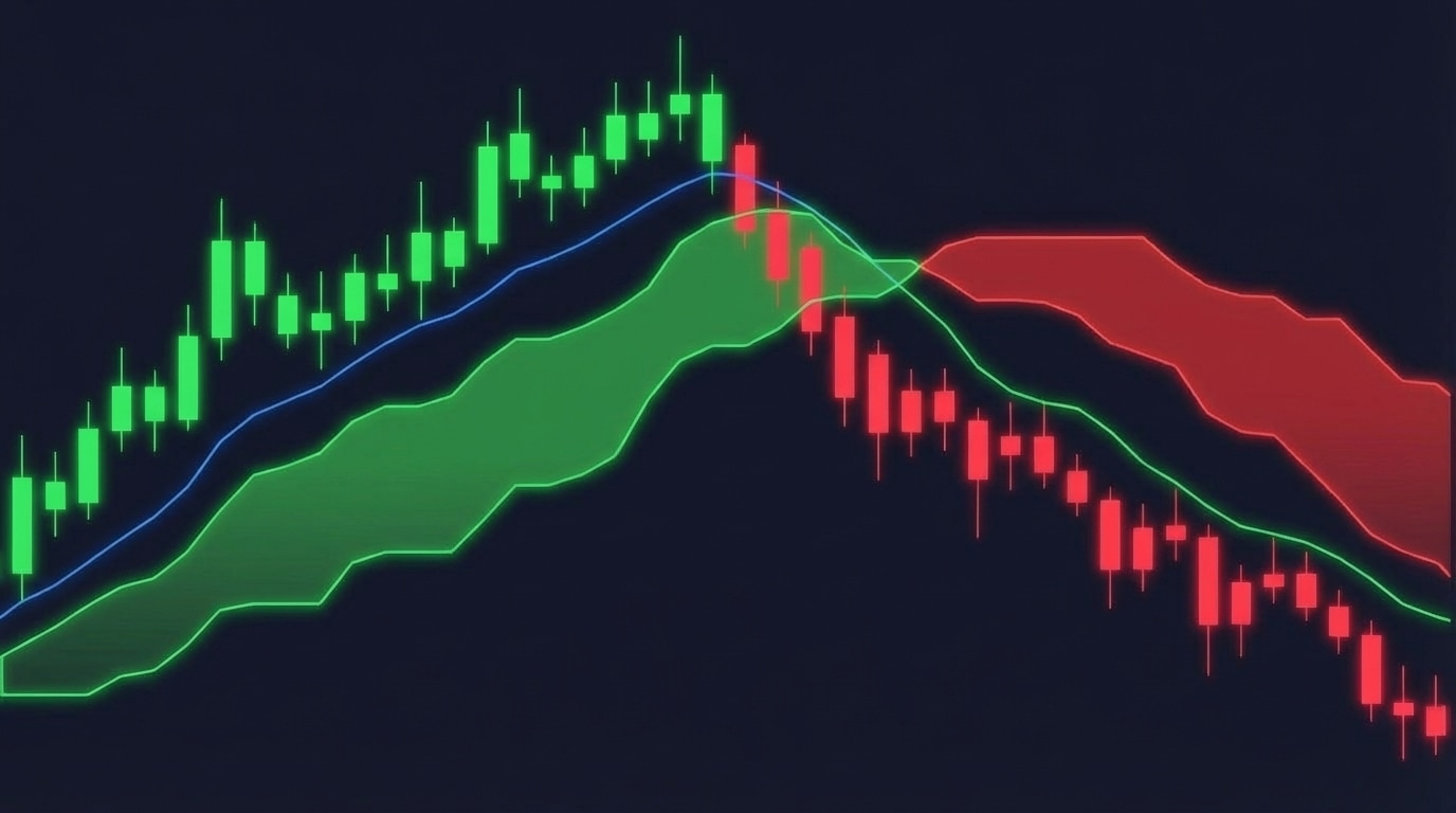
We now combine the EMA trend filter with Ichimoku cloud conditions to find high-probability entries.

Entry Rules for LONG Position

Step 1: Confirm Uptrend (EMA Filter)

EMA_signal == +1 (at least 7 candles fully above EMA 100)

Step 2: Confirm Momentum (Ichimoku Cloud)

Within the last 10 candles, at least 7 must be FULLY ABOVE the cloud

“Fully above” means: Open > cloud_top AND Close > cloud_top

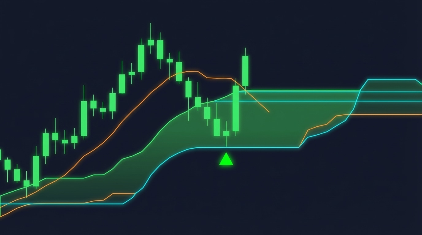
Step 3: The Entry Trigger (Cloud Pierce)

Current candle opens INSIDE the cloud AND closes ABOVE it

This represents a retracement that is bouncing back into the trend direction.

Entry Rules for SHORT Position

Mirror image:

  1. EMA_signal == -1
  2. At least 7 of 10 candles fully BELOW cloud
  3. Current candle opens inside cloud, closes BELOW

Why These Rules Work

“We are trading with a trend and we are trying to capture patterns where candles are also above the Ichimoku cloud confirming a strong momentum. But then we look for a candle dipping or bouncing in and out of the cloud because we are looking for some kind of a retracement.”

The key insight:

“When the candle closes above the cloud, we assume that the retracement is over and the price will probably continue in the direction of the main trend.”

Code Implementation

def createSignals(df: pd.DataFrame,
                  lookback_window: int = 10,
                  min_confirm: int = 5,
                  ema_signal_col: str = "EMA_signal") -> pd.DataFrame:
    """
    Produce a single signal column aligned with EMA trend:
      +1 (long):  Ichimoku pierce-up + enough prior bars entirely ABOVE cloud
                   AND EMA_signal == +1
      -1 (short): Ichimoku pierce-down + enough prior bars entirely BELOW cloud
                   AND EMA_signal == -1
       0 (none): otherwise
    """
    out = df.copy()
    
    # Cloud boundaries
    cloud_top = out[["ich_spanA", "ich_spanB"]].max(axis=1)
    cloud_bot = out[["ich_spanA", "ich_spanB"]].min(axis=1)
    
    # Candles entirely above/below cloud
    above_cloud = (out["Open"] > cloud_top) & (out["Close"] > cloud_top)
    below_cloud = (out["Open"] < cloud_bot) & (out["Close"] < cloud_bot)
    
    above_count = above_cloud.rolling(lookback_window, min_periods=lookback_window).sum()
    below_count = below_cloud.rolling(lookback_window, min_periods=lookback_window).sum()
    
    # Current-bar pierce conditions
    pierce_up   = (out["Open"] < cloud_top) & (out["Close"] > cloud_top)
    pierce_down = (out["Open"] > cloud_bot) & (out["Close"] < cloud_bot)
    
    # Trend confirmations
    up_trend_ok   = above_count >= min_confirm
    down_trend_ok = below_count >= min_confirm
    
    # EMA alignment
    ema_up   = (out[ema_signal_col] == 1)
    ema_down = (out[ema_signal_col] == -1)
    
    # Final conditions
    long_cond  = up_trend_ok & pierce_up & ema_up
    short_cond = down_trend_ok & pierce_down & ema_down
    
    signal = np.where(long_cond & ~short_cond,  1,
             np.where(short_cond & ~long_cond, -1, 0)).astype(int)
    
    out["signal"] = signal
    return out

# Usage
df = createSignals(df, lookback_window=10, min_confirm=7)

Ideal vs Non-Ideal Entries

Ideal Entry

  • Small candle that dips into cloud
  • Closes just above cloud top
  • Three long wicks showing rejection of cloud (support)
  • Tight entry close to cloud = better risk/reward

Less Ideal Entry

  • Long candle that dips into cloud
  • Closes far above cloud top
  • Entry is “late” = wider stop-loss needed

Coming Up Next: We know when to enter — now let us protect our capital with proper trade management. Continue to Part 6 →

EMA Trend Filter for Ichimoku Trading

EMA Trend Filter
The EMA 100 trend filter ensures we only trade in the direction of the prevailing trend

Ichimoku Trading Series: Part 4 of 10 | ← Previous | View Full Series

Why Add an EMA Filter?

The Ichimoku Cloud alone can generate signals in choppy markets. The EMA filter ensures we only trade when a clear trend is established.

The Rule: EMA 100

We use a 100-period Exponential Moving Average as our trend identifier.

Long Trend Conditions

Current candle + at least 5 previous candles ALL trading FULLY ABOVE the EMA

“Fully above” means:

  • Open > EMA
  • Close > EMA

Short Trend Conditions

Current candle + at least 5 previous candles ALL trading FULLY BELOW the EMA

Why 5+ Candles?

From the source material:

“We need the current candle plus at least five previous candles all trading fully above the EMA curve. Meaning both the open and close of each of these candles are above the line.”

This confirms we are in a sustained trend, not just a momentary spike.

Code Implementation

def MovingAverageSignal(df: pd.DataFrame, back_candles: int = 5) -> pd.DataFrame:
    """
    Add a single-column EMA trend signal to the DataFrame.

    Rules (evaluated per bar, using *only* current/past data):
      +1 (uptrend):   For the window [t-back_candles .. t], EVERY bar has
                      Open > EMA and Close > EMA.
      -1 (downtrend): For the same window, EVERY bar has
                      Open < EMA and Close < EMA.
       0 otherwise.
    """
    out = df.copy()
    
    # Window size: current bar + back_candles bars behind it
    w = int(back_candles) + 1
    
    # Booleans per-bar relative to EMA
    above = (out["Open"] > out["EMA"]) & (out["Close"] > out["EMA"])
    below = (out["Open"] < out["EMA"]) & (out["Close"] < out["EMA"])
    
    # "All true in the last w bars" via rolling sum == w
    above_all = (above.rolling(w, min_periods=w).sum() == w)
    below_all = (below.rolling(w, min_periods=w).sum() == w)
    
    # Single signal column
    signal = np.where(above_all, 1, np.where(below_all, -1, 0)).astype(int)
    out["EMA_signal"] = signal
    
    return out

# Usage: require 7 candles above/below EMA
df = MovingAverageSignal(df, back_candles=7)

Tuning the Parameter

Setting Effect
back_candles=5 More signals, less trend confirmation
back_candles=7 Balanced (recommended)
back_candles=10 Fewer signals, stronger trend confirmation

Coming Up Next: In Part 5, we will define our exact entry conditions — when the EMA trend is confirmed AND the Ichimoku cloud gives us a retracement signal. Continue to Part 5 →

Understanding the Kumo Cloud

Understanding the Kumo Cloud
Bullish and bearish cloud formations with price piercing through

Ichimoku Trading Series: Part 3 of 10 | ← Previous | View Full Series

The Cloud (Kumo)

The space between Senkou Span A and Senkou Span B creates the “cloud” — a dynamic zone of support and resistance.

Bullish Cloud (Green)

When Span A > Span B, the cloud is bullish:

Price → [Span A (top)] → [Span B (bottom)]

Bearish Cloud (Red)

When Span B > Span A, the cloud is bearish:

Price → [Span B (top)] → [Span A (bottom)]

What the Cloud Tells Us

1. Trend Direction

  • Price above cloud = Bullish trend
  • Price below cloud = Bearish trend
  • Price inside cloud = Consolidation/uncertainty

2. Support/Resistance Strength

  • Thick cloud = Strong support/resistance
  • Thin cloud = Weak support/resistance, easier breakouts

3. Future Sentiment

The cloud projects forward, showing where support/resistance WILL BE.

Critical: Avoiding Look-Ahead Bias

The Problem

Standard Ichimoku implementations shift Span A and Span B 26 periods into the future. In backtesting, this means your strategy “knows” future support/resistance levels — data leakage!

Our Solution

# We use UNshifted spans for signal logic
span_a_raw = (tenkan_line + kijun_line) / 2.0  # raw (no forward shift)
span_b_raw = (h.rolling(senkou_b).max() + l.rolling(senkou_b).min()) / 2.0  # raw

From the source material:

“I decided to compute the Ichimoku manually for one reason… The Ichimoku by default shifts or reads a bit in the future. This would be a look-ahead bias for our backtesting.”

Cloud Boundaries for Signals

cloud_top = df[["ich_spanA", "ich_spanB"]].max(axis=1)
cloud_bot = df[["ich_spanA", "ich_spanB"]].min(axis=1)

Cloud Twist

When the cloud changes colour (Span A and Span B cross), it signals a potential trend reversal. This is called a Kumo Twist or Senkou Span Cross.

  • Bullish Twist: Span A crosses above Span B → Cloud turns green
  • Bearish Twist: Span A crosses below Span B → Cloud turns red

Coming Up Next: The cloud tells us about support and resistance, but we need a trend filter to avoid false signals. In Part 4, we add our EMA Trend Filter. Continue to Part 4 →

The Five Ichimoku Components Explained

The Five Ichimoku Components
The five sacred lines of Ichimoku Kinko Hyo

Ichimoku Trading Series: Part 2 of 10 | ← Previous | View Full Series

The Sacred Five Lines

Ichimoku Kinko Hyo (一目均衡表) translates to “one glance equilibrium chart” — a complete trading system visible at a glance.

1. Tenkan-sen (Conversion Line) — Period: 9

tenkan = (highest_high_9 + lowest_low_9) / 2

The fastest-moving line, representing short-term momentum.

Trading Insight: When Tenkan crosses above Kijun, it is bullish. Below = bearish.

2. Kijun-sen (Base Line) — Period: 26

kijun = (highest_high_26 + lowest_low_26) / 2

The medium-term equilibrium. Price tends to return to this line.

Trading Insight: Acts as dynamic support/resistance. A flat Kijun indicates consolidation.

3. Senkou Span A (Leading Span A)

span_a = (tenkan + kijun) / 2
# Traditionally plotted 26 periods ahead

The faster of the two cloud boundaries.

4. Senkou Span B (Leading Span B) — Period: 52

span_b = (highest_high_52 + lowest_low_52) / 2
# Traditionally plotted 26 periods ahead

The slower, more stable cloud boundary.

5. Chikou Span (Lagging Span)

chikou = close  # Plotted 26 periods BEHIND

Current price shown lagged for momentum confirmation.

The Parameters

Component Default Period Our Setting
Tenkan 9 9
Kijun 26 26
Senkou B 52 52

These are the original parameters developed for Japanese rice markets in the 1930s. They translate to roughly:

  • 9 = 1.5 trading weeks
  • 26 = 1 trading month
  • 52 = 2 trading months

Code Implementation

# Ichimoku params (defaults)
TENKAN       = 9
KIJUN        = 26
SENKOU_B     = 52

How the Lines Interact

TK Cross (Tenkan/Kijun Cross)

  • Bullish: Tenkan crosses ABOVE Kijun
  • Bearish: Tenkan crosses BELOW Kijun
  • Strongest: When cross happens above the cloud (bullish) or below (bearish)

Chikou Confirmation

  • Bullish: Chikou is above price from 26 periods ago
  • Bearish: Chikou is below price from 26 periods ago

Coming Up Next: In Part 3, we will explore the Kumo Cloud itself — how to read bullish vs bearish clouds and why cloud thickness matters. Continue to Part 3 →

Introduction to Ichimoku Cloud Trading

Ichimoku Cloud Trading Strategy Overview
The Ichimoku Cloud combined with EMA trend filtering creates high-probability trade setups

Ichimoku Trading Series: Part 1 of 10 | View Full Series

What You Will Build

In this 10-part series, you will learn to automate a trading strategy that combines:

  • Ichimoku Cloud (Ichimoku Kinko Hyo) for entry signals
  • EMA 100 as a trend filter
  • ATR-based stop-loss and take-profit management

The strategy achieved ~40% yearly returns in backtests across multiple FX pairs on the 4-hour timeframe, with a 53-69% win rate and controlled drawdowns.

Why This Strategy Works

The core principle is simple but powerful:

  1. Trade WITH the trend — The EMA filter ensures we only take trades in the prevailing market direction
  2. Wait for retracements — The Ichimoku Cloud identifies perfect pullback entries
  3. Enter at the bounce — When price dips INTO the cloud and closes OUTSIDE, the retracement is likely over

Visual Signal Example

Green triangles = Long signals (buy)
Red triangles = Short signals (sell)

The strategy only takes trades that align with both the EMA trend AND the Ichimoku setup.

What Makes This Approach Unique

Problem with Standard Ichimoku

Most Ichimoku implementations suffer from look-ahead bias — they shift the cloud forward in time, which gives misleadingly good backtest results.

Our Solution

We compute the Ichimoku components without forward-shifting the spans, ensuring honest backtesting results that translate to real trading.

Key Backtest Results

Metric Value
Annual Return 28-43%
Win Rate 53-69%
Max Drawdown -6% to -21%
Sharpe Ratio 1.0-1.38
Trades per Year ~13 (selective)

Important Note: The strategy is SELECTIVE — only ~13 trades per year. This is a feature, not a bug. Quality over quantity.

Course Overview

Over the next 10 parts, you will learn:

  • Part 2: The Five Ichimoku Components
  • Part 3: Understanding the Kumo Cloud
  • Part 4: EMA Trend Filter
  • Part 5: Entry Signal Conditions
  • Part 6: Trade Management with ATR
  • Part 7: Python Backtesting Setup
  • Part 8: Building the Strategy Class
  • Part 9: Parameter Optimisation
  • Part 10: Results Analysis & Next Steps

Prerequisites

  • Basic Python knowledge
  • Understanding of candlestick charts
  • Familiarity with trading concepts (SL, TP, R:R)

Coming Up Next: In Part 2, we will dive deep into the five Ichimoku components and understand exactly what each line tells us about market structure. Continue to Part 2 →

Concept Vectors and Analogy in LLMs

LLM Architecture Series – Bonus Lesson. In earlier lessons you saw how tokens become vectors. This article goes deeper into what those vectors mean and how simple arithmetic on them can reveal structure in concepts.

Concept vectors in embedding space

Concept vectors in embedding space, generated with Nano Banana.

(more…)

The Complete LLM Pipeline – Putting It All Together

LLM Architecture Series – Lesson 20 of 20. We have visited every component of the architecture. This lesson ties them together into a single mental model.

By walking through a full end to end example you can see how tokenization, embeddings, attention, MLPs, and the output layer cooperate to produce text.

(more…)

Scaling LLMs – nano-GPT to GPT-3

LLM Architecture Series – Lesson 19 of 20. You now understand the core architecture. Scaling is about what happens when we make models wider, deeper, and train them on more data.

Surprisingly, performance often follows smooth scaling laws, which lets practitioners predict the benefit of using larger models.

(more…)

From Logits to Probabilities – Softmax Output

LLM Architecture Series – Lesson 18 of 20. The output layer produces one logit per token in the vocabulary. Softmax converts these logits into a proper probability distribution.

These probabilities drive sampling strategies such as greedy decoding, top k sampling, and nucleus sampling.

(more…)

The Output Layer and Language Model Head

LLM Architecture Series – Lesson 17 of 20. After many transformer layers, we have a final hidden vector for each position. The output layer turns this into raw scores for every token in the vocabulary.

This linear layer is often called the language model head and is where most parameters of the model live.

(more…)