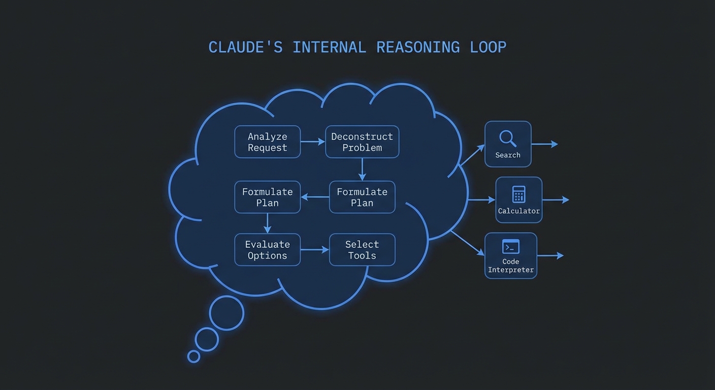
Claude Code is Anthropic’s autonomous coding agent – and it is built on MCP. When Claude Code reads files, runs tests, executes commands, and browses documentation, it does all of this through MCP servers. The architecture is not a coincidence: it is Anthropic demonstrating exactly how a production-grade autonomous agent should integrate with external systems. Understanding how Claude Code uses MCP is one of the fastest ways to understand how you should build your own agents.
Claude Code’s MCP Architecture
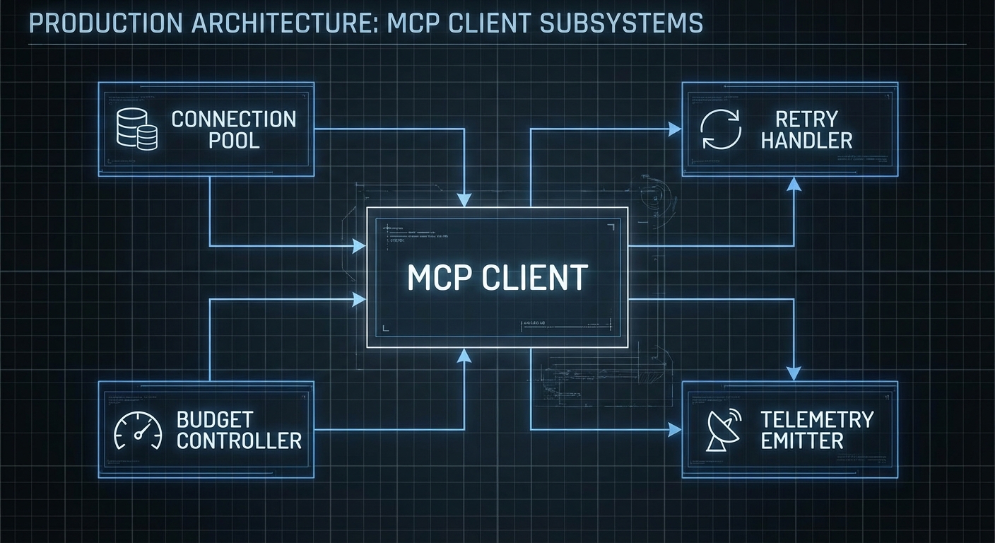
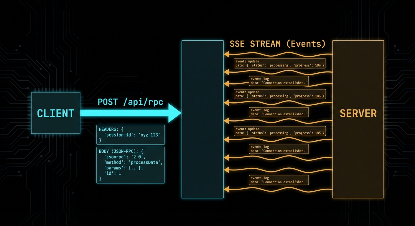
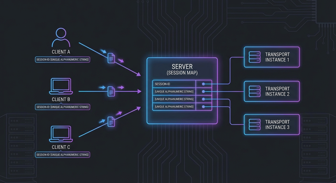
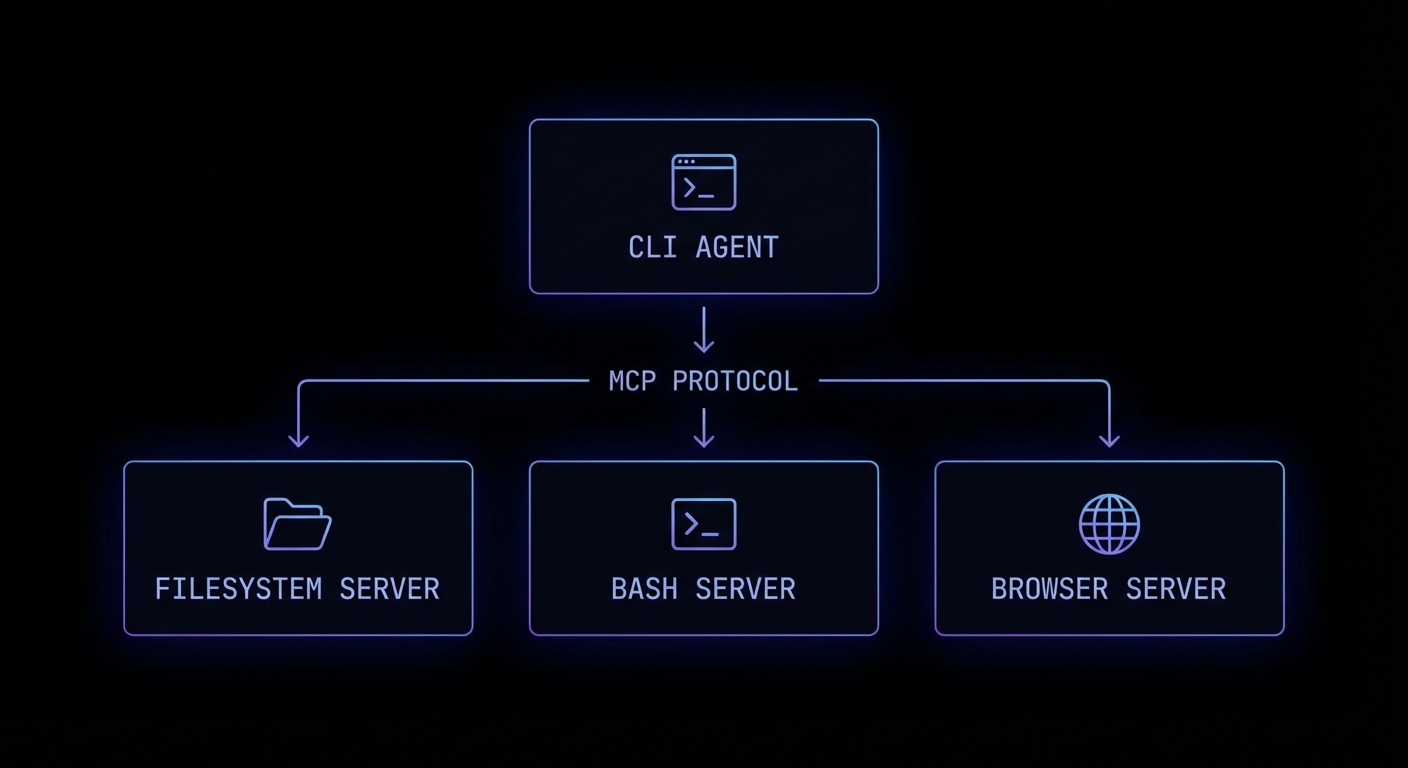
Claude Code (the CLI tool, claude) operates as an MCP host. When it starts, it connects to a set of built-in MCP servers that provide its core capabilities: computer-use (screen reading/clicking), bash (shell command execution), and files (filesystem read/write). You can extend Claude Code with your own custom MCP servers, making it immediately capable of working with your specific project tools.
# ~/.claude/config.json - Extend Claude Code with your MCP servers
{
  "mcpServers": {
    "my-project-tools": {
      "command": "node",
      "args": ["./tools/mcp-server.js"],
      "env": {
        "DATABASE_URL": "postgresql://localhost/mydb"
      }
    },
    "github-tools": {
      "command": "npx",
      "args": ["-y", "@anthropic-ai/mcp-github"]
    }
  }
}
Once configured, Claude Code can use your custom server’s tools as naturally as it uses its built-in bash or filesystem tools. Your create_github_issue tool becomes as usable as Bash(git commit).
Building Agent Skills for Claude Code
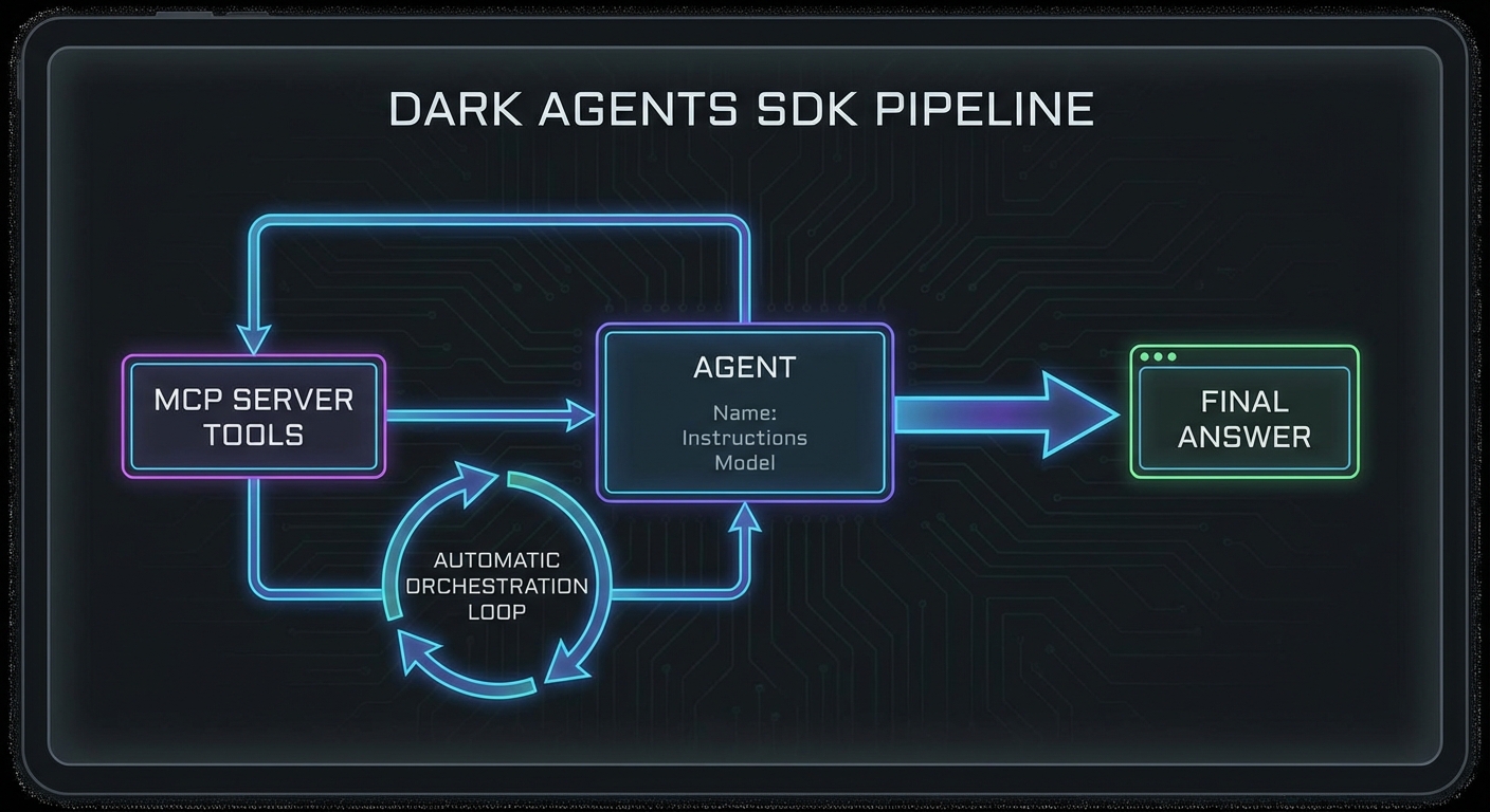
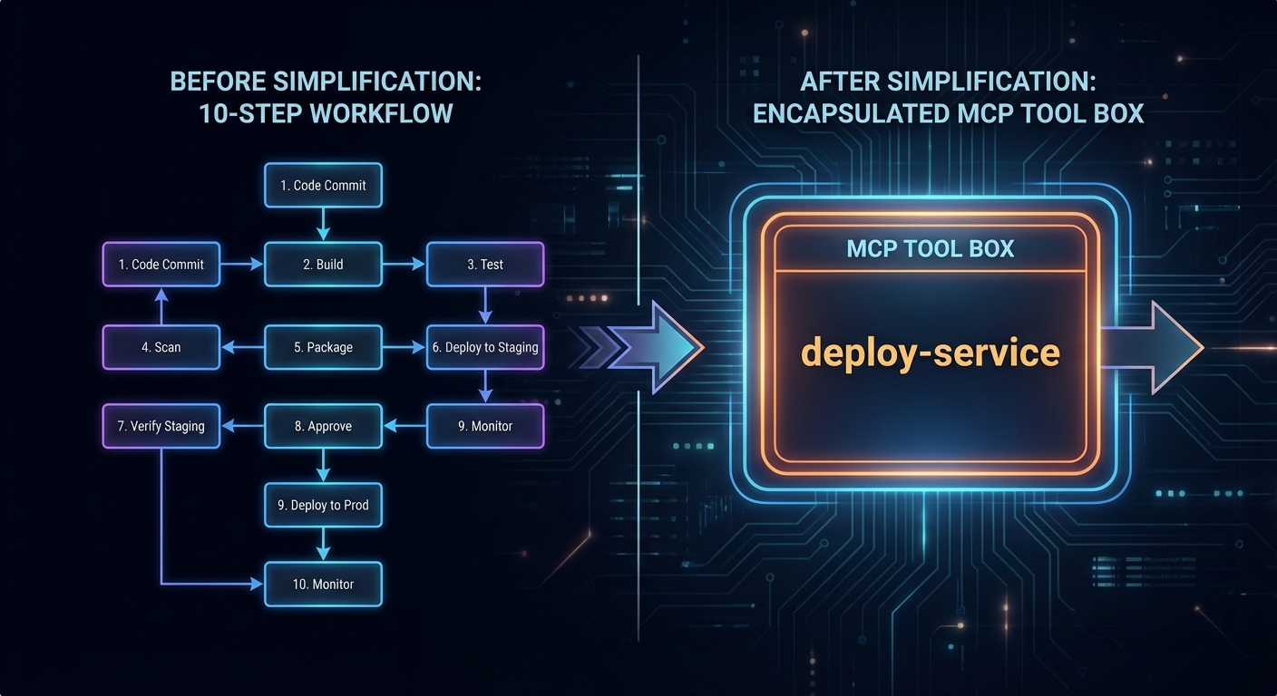
The most powerful Claude Code extension pattern is the “agent skill” – a specialised MCP server that encapsulates a complex workflow as a single callable tool. Instead of Claude figuring out the 20-step process to deploy a microservice, you encode those steps in a deploy_service tool that handles all the complexity.
// deploy-skill-server.js
import { McpServer } from '@modelcontextprotocol/sdk/server/mcp.js';
import { StdioServerTransport } from '@modelcontextprotocol/sdk/server/stdio.js';
import { z } from 'zod';
import { execFile } from 'node:child_process';
import { promisify } from 'node:util';

const exec = promisify(execFile);
const server = new McpServer({ name: 'deploy-skills', version: '1.0.0' });

server.tool(
  'deploy_service',
  `Deploy a microservice to Kubernetes. Handles build, push, and rollout.
  Returns the deployment status and the new pod count.`,
  {
    service_name: z.string().describe('Name of the service to deploy'),
    image_tag: z.string().describe('Docker image tag to deploy'),
    namespace: z.string().default('production').describe('Kubernetes namespace'),
    replicas: z.number().int().min(1).max(10).default(2),
  },
  async ({ service_name, image_tag, namespace, replicas }) => {
    const steps = [];

    // Step 1: Build
    const { stdout: buildOut } = await exec('docker', [
      'build', '-t', `${service_name}:${image_tag}`, './services/' + service_name
    ]);
    steps.push('Build: OK');

    // Step 2: Push
    await exec('docker', ['push', `myregistry/${service_name}:${image_tag}`]);
    steps.push('Push: OK');

    // Step 3: Deploy
    const manifest = generateK8sManifest(service_name, image_tag, namespace, replicas);
    await exec('kubectl', ['apply', '-f', '-'], { input: manifest });
    steps.push(`Deploy: OK (${replicas} replicas)`);

    // Step 4: Wait for rollout
    await exec('kubectl', ['rollout', 'status', `deployment/${service_name}`, '-n', namespace]);
    steps.push('Rollout: Complete');

    return {
      content: [{ type: 'text', text: steps.join('\n') + `\n\nService ${service_name} deployed successfully.` }],
    };
  }
);

const transport = new StdioServerTransport();
await server.connect(transport);
Permission Modes in Claude Code
Claude Code has a permission system that controls what actions it can take without asking for confirmation. MCP tools are subject to the same permission model. You can configure Claude Code to auto-approve specific tools, require confirmation for destructive operations, or run in fully supervised mode.
# .claude/settings.json (project-level)
{
  "permissions": {
    "allow": [
      "Bash(git *)",              # Allow all git commands
      "mcp:my-project-tools:read_*",  # Allow read-only tools from my server
      "Read(**)"                   # Allow reading any file
    ],
    "deny": [
      "mcp:my-project-tools:deploy_*",  # Always ask before deploying
      "Bash(rm -rf *)"            # Never auto-approve recursive deletes
    ]
  }
}
“Claude Code is designed to be an autonomous coding agent that can understand and work on complex codebases. It uses a set of built-in tools and can be extended with custom MCP servers to access domain-specific capabilities.” – Anthropic Documentation, Claude Code
Failure Modes with Claude Code MCP Extensions
Case 1: Tools That Are Too Granular
// BAD: Too granular - Claude has to call many tools in sequence and may make mistakes
server.tool('set_k8s_namespace', '...', { ns: z.string() }, handler);
server.tool('set_k8s_image', '...', { image: z.string() }, handler);
server.tool('apply_k8s_manifest', '...', { manifest: z.string() }, handler);
server.tool('watch_k8s_rollout', '...', { deployment: z.string() }, handler);

// BETTER: One atomic skill tool that handles the whole workflow
server.tool('deploy_service', 'Deploy a service to k8s...', { service: z.string(), ... }, handler);
Case 2: Forgetting to Handle Long-Running Operations
// Build + deploy can take minutes
// Don't timeout. Stream progress via notifications or use progress indicators
// Claude Code will wait, but it needs feedback to know the tool is running

server.tool('build_and_deploy', '...', { ... }, async ({ service }) => {
  // Send progress
  process.stderr.write(`[build] Starting build for ${service}...\n`);
  await buildService(service);  // May take 2-10 minutes
  process.stderr.write(`[deploy] Deploying ${service}...\n`);
  await deployService(service);
  return { content: [{ type: 'text', text: 'Done.' }] };
});
What to Check Right Now
- Install Claude Code –
npm install -g @anthropic-ai/claude-code. Then runclaudein a project directory to see it in action. - Add your MCP server to Claude Code config – add it to
~/.claude/config.jsonor.claude/config.json(project-level). Then runclaudeand ask it to use your tool. - Design tools as atomic workflows – each tool should complete one meaningful unit of work end-to-end. Avoid exposing low-level implementation details as separate tools.
- Review the permission system – set appropriate
allowanddenyrules for your project. Deny destructive tools by default and require explicit confirmation.
nJoy 😉