Tool calling with a single round-trip response is the entry point. But production MCP applications need streaming – the ability to show intermediate results to users as the model thinks – and structured outputs, which guarantee that the model’s final answer conforms to a schema you define. This lesson adds both to your OpenAI + MCP integration, covering the streaming tool call parsing mechanics and the structured output patterns that prevent hallucinated schemas in production.
Streaming with Tool Calls
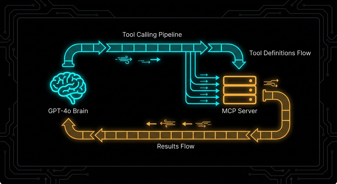
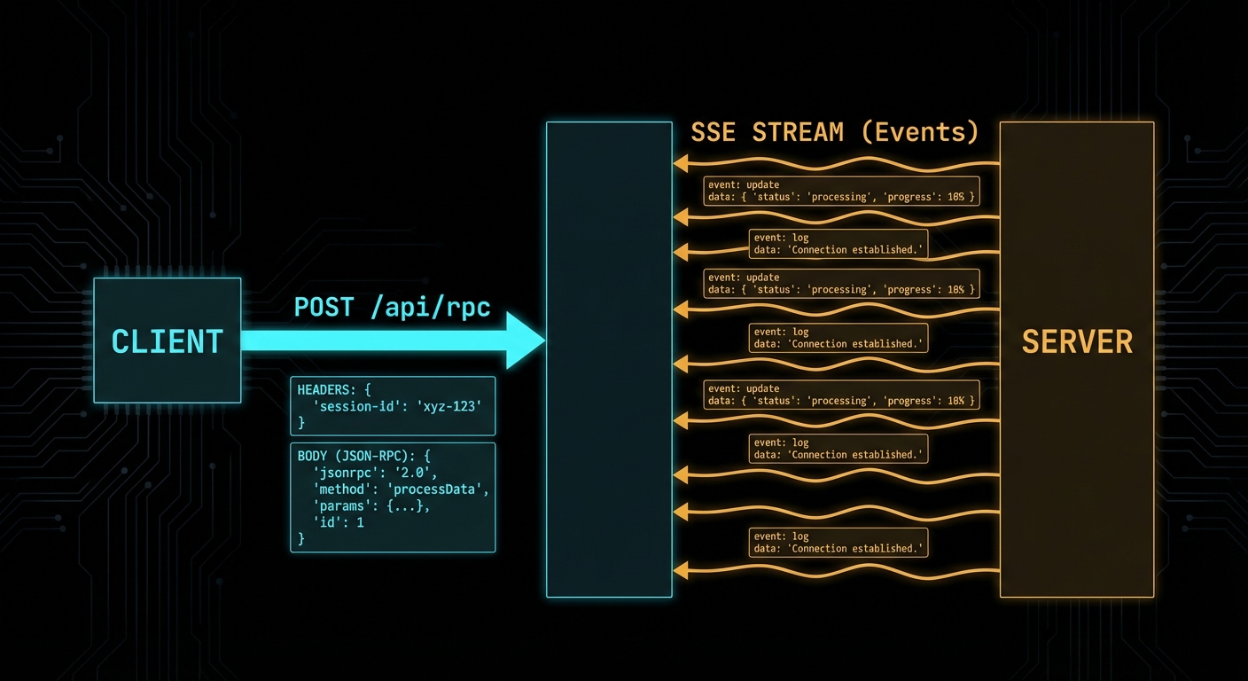
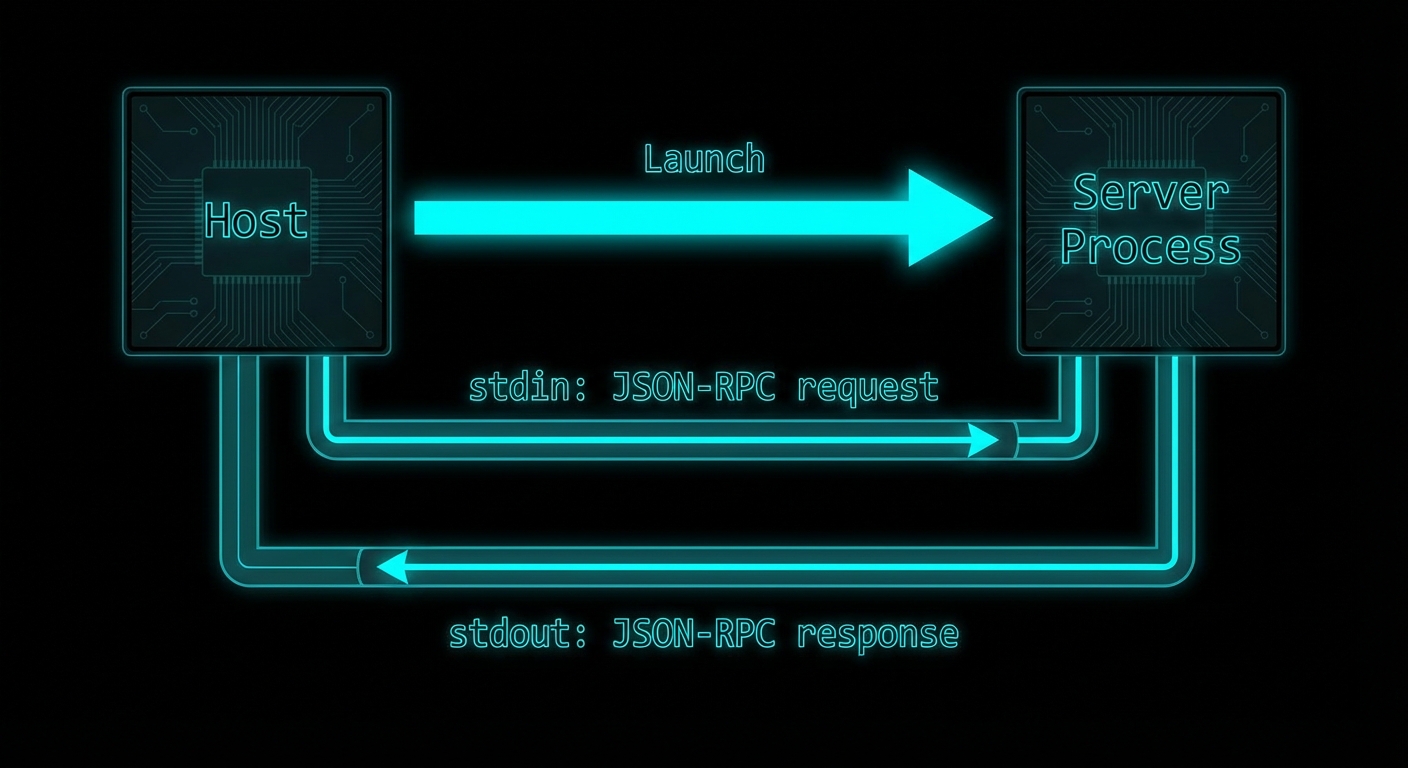
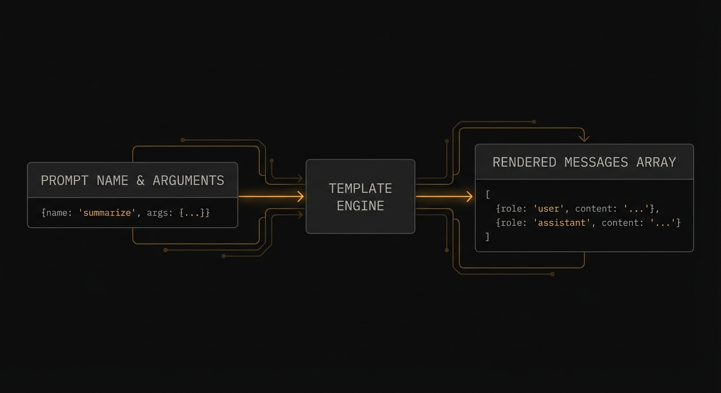
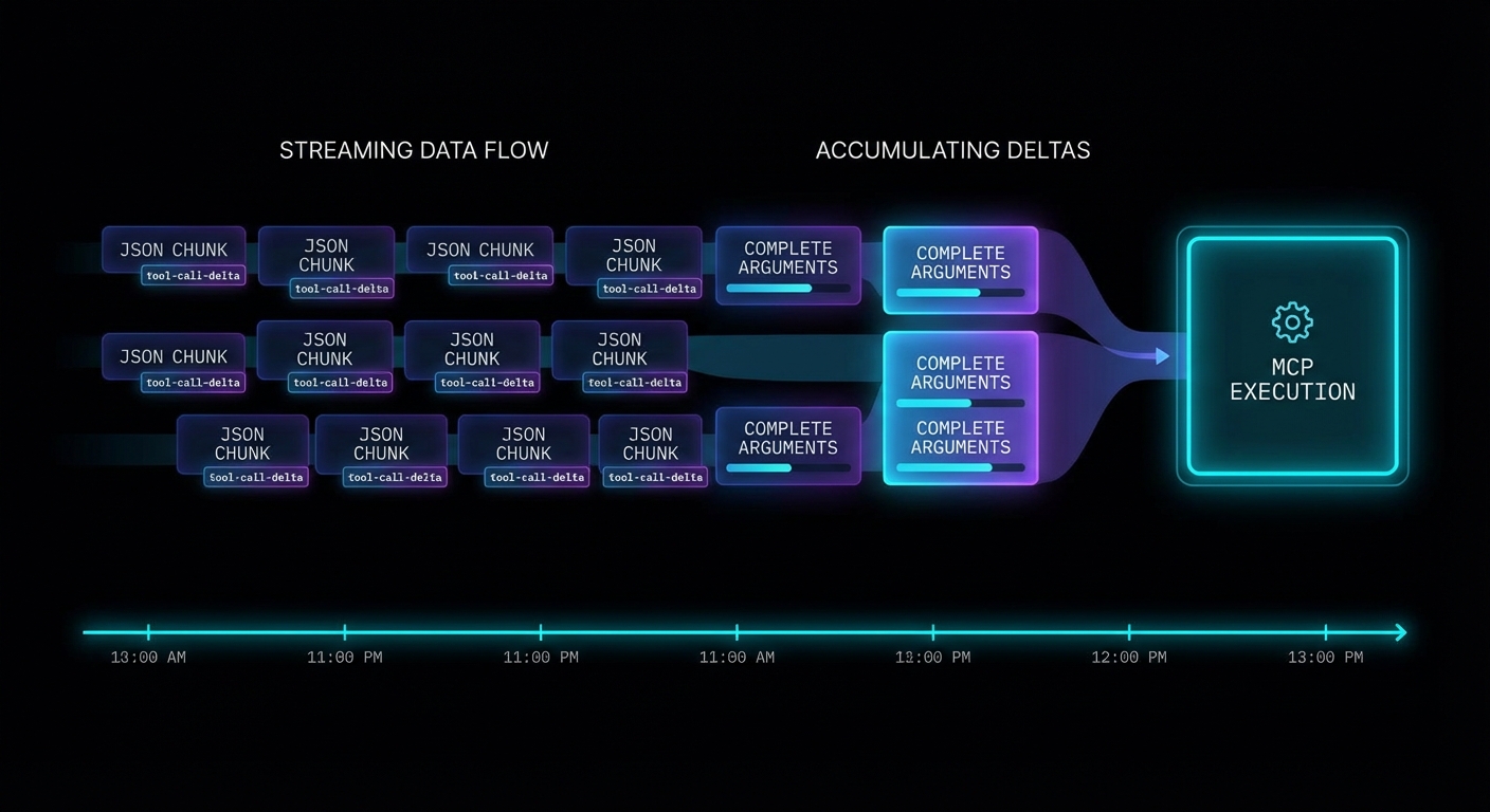
When you stream a completion that includes tool calls, the tool call arguments arrive incrementally as delta chunks. You must accumulate them before you can parse and execute the tool. The pattern is: buffer all deltas, detect when a tool call is complete, then execute through MCP.
import OpenAI from 'openai';
import { Client } from '@modelcontextprotocol/sdk/client/index.js';
import { StdioClientTransport } from '@modelcontextprotocol/sdk/client/stdio.js';
const openai = new OpenAI({ apiKey: process.env.OPENAI_API_KEY });
const mcpClient = new Client({ name: 'streaming-host', version: '1.0.0' }, { capabilities: {} });
await mcpClient.connect(new StdioClientTransport({ command: 'node', args: ['server.js'] }));
const { tools: mcpTools } = await mcpClient.listTools();
const openAITools = mcpTools.map(t => ({
type: 'function',
function: { name: t.name, description: t.description, parameters: t.inputSchema },
}));
async function runStreamingWithTools(userMessage) {
const messages = [{ role: 'user', content: userMessage }];
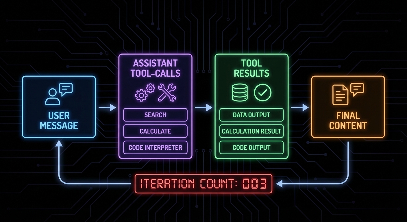
while (true) {
// Stream the completion
const stream = await openai.chat.completions.create({
model: 'gpt-4o',
messages,
tools: openAITools,
stream: true,
});
// Accumulate the full response
let assistantMessage = { role: 'assistant', content: '', tool_calls: [] };
const toolCallMap = {}; // index -> accumulated tool call
for await (const chunk of stream) {
const delta = chunk.choices[0]?.delta;
if (!delta) continue;
// Stream text content to UI
if (delta.content) {
assistantMessage.content += delta.content;
process.stdout.write(delta.content); // Real-time output
}
// Accumulate tool call deltas
if (delta.tool_calls) {
for (const tcDelta of delta.tool_calls) {
const idx = tcDelta.index;
if (!toolCallMap[idx]) {
toolCallMap[idx] = { id: '', type: 'function', function: { name: '', arguments: '' } };
}
const tc = toolCallMap[idx];
if (tcDelta.id) tc.id += tcDelta.id;
if (tcDelta.function?.name) tc.function.name += tcDelta.function.name;
if (tcDelta.function?.arguments) tc.function.arguments += tcDelta.function.arguments;
}
}
}
assistantMessage.tool_calls = Object.values(toolCallMap);
messages.push(assistantMessage);
// No tool calls = we have the final answer
if (assistantMessage.tool_calls.length === 0) {
return assistantMessage.content;
}
// Execute all accumulated tool calls through MCP
const toolResults = await Promise.all(
assistantMessage.tool_calls.map(async (tc) => {
const args = JSON.parse(tc.function.arguments);
console.error(`\n[tool] Calling: ${tc.function.name}`);
const result = await mcpClient.callTool({ name: tc.function.name, arguments: args });
const text = result.content.filter(c => c.type === 'text').map(c => c.text).join('\n');
return { role: 'tool', tool_call_id: tc.id, content: text };
})
);
messages.push(...toolResults);
}
}
const answer = await runStreamingWithTools('What are the best products under $50?');
console.log('\n\nFinal:', answer);
Structured Outputs with MCP Tool Results
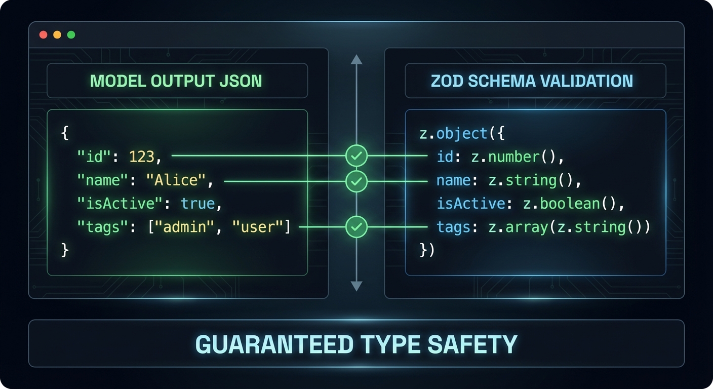
OpenAI’s structured outputs feature forces the model to return JSON that exactly matches a schema you specify. This is different from JSON mode (which just returns valid JSON) – structured outputs guarantee that every required field is present and every value is the correct type. You can use structured outputs for the final answer even when intermediate steps use tool calls.
import { z } from 'zod';
import { zodResponseFormat } from 'openai/helpers/zod.js';

// Define the schema for the final answer
const ProductRecommendationSchema = z.object({
  recommendations: z.array(z.object({
    product_name: z.string(),
    price: z.number(),
    reason: z.string(),
    confidence: z.enum(['high', 'medium', 'low']),
  })),
  total_products_checked: z.number(),
  search_strategy: z.string(),
});

// Use structured output for the final response
const finalResponse = await openai.beta.chat.completions.parse({
  model: 'gpt-4o',
  messages: [
    ...conversationHistory,
    { role: 'user', content: 'Based on the search results, provide your top 3 recommendations.' },
  ],
  response_format: zodResponseFormat(ProductRecommendationSchema, 'product_recommendations'),
});

const recommendations = finalResponse.choices[0].message.parsed;
// recommendations is now typed as ProductRecommendation - guaranteed to match schema
console.log(recommendations.recommendations[0].product_name);
“Structured Outputs is a feature that ensures the model will always generate responses that adhere to your supplied JSON Schema, so you don’t need to worry about the model omitting a required key, or hallucinating an invalid enum value.” – OpenAI Documentation, Structured Outputs
Failure Modes with Streaming Tool Calls
Case 1: Parsing Arguments Before All Deltas Arrive
// WRONG: Parsing tool call arguments during streaming
for await (const chunk of stream) {
  const delta = chunk.choices[0]?.delta;
  if (delta.tool_calls?.[0]?.function?.arguments) {
    const args = JSON.parse(delta.tool_calls[0].function.arguments); // WRONG - may be partial JSON
    await mcpClient.callTool({ ... });
  }
}

// CORRECT: Accumulate all deltas first, then parse
// (As shown in the complete streaming loop above)
Case 2: Missing tool_call_id in Tool Result Messages
// WRONG: tool_call_id missing or mismatched
messages.push({ role: 'tool', content: result }); // Missing tool_call_id

// CORRECT: Each tool result must include the exact tool_call_id
messages.push({ role: 'tool', tool_call_id: tc.id, content: result });
What to Check Right Now
- Test streaming with a multi-tool query – ask a question that forces two tool calls in sequence. Verify the streaming output is coherent and the final answer is correct.
- Add a progress indicator – during streaming, show a spinner or partial text. Users should see something happening, not a blank screen for 10 seconds.
- Use structured outputs for all final answers – wherever your application needs to parse the model’s response programmatically, use structured outputs. It eliminates an entire class of parsing bugs.
- Handle stream errors – wrap the
for await (const chunk of stream)loop in a try-catch. Network errors during streaming are common and need graceful handling.
nJoy 😉