
Google just published a compression algorithm so efficient that it sent memory chip stocks tumbling across three continents in a single trading session. SK Hynix down 6%. Samsung down 5%. Micron bleeding for six days straight. Billions of dollars in market capitalisation evaporated because a team of researchers figured out a cleverer way to point at things. That is not a metaphor. That is literally what they did. Welcome to TurboQuant, the algorithm that halves the cost of running every large language model on the planet, and the wildest part is that Google just gave it away for free.

What the KV Cache Actually Is (And Why Everyone Should Care)
Before we get into what Google built, you need to understand the bottleneck they solved. Every large language model, whether it is ChatGPT, Claude, Gemini, or Llama, runs on the transformer architecture. And transformers have this mechanism called attention, which is how the model figures out what words mean in context.
Here is a quick thought experiment. If I say “it was tired,” you have no idea what “it” refers to. A dog? A server? A metaphor for the state of modern JavaScript? But if I say “the animal didn’t cross the street because it was too tired,” suddenly “it” is loaded with meaning. It is an animal. It didn’t cross. It was tired. Your brain just did what transformers do: it looked at the surrounding words to figure out what one word actually means.
The problem is that transformers need to remember these relationships. Every time the model processes a token, it calculates how that token relates to every other token it has seen so far. These relationships get stored in what is called the key-value cache (KV cache). Think of it as a filing cabinet. Each “folder” has a label on the front (the key, which is a rough tag so the model can find it quickly) and detailed notes inside (the value, which is the actual rich meaning and relationships).
The catch? This filing cabinet grows linearly with context length. A 128K context window means 128,000 tokens worth of folders, each containing high-dimensional vectors stored at 16-bit precision. For a model like Llama 3.1 with 8 billion parameters, the KV cache alone can eat several gigabytes of GPU memory. For larger models with longer contexts, it becomes the single biggest memory bottleneck in the entire inference pipeline. Not the model weights. Not the activations. The KV cache.
“Vector quantization is a powerful, classical data compression technique that reduces the size of high-dimensional vectors. This optimization addresses two critical facets of AI: it enhances vector search […] and it helps unclog key-value cache bottlenecks by reducing the size of key-value pairs.” — Google Research, TurboQuant Blog Post (March 2026)
Traditional approaches to compressing the KV cache use something called quantisation, which reduces the precision of the stored numbers. Instead of 16 bits per value, you use 8 bits, or 4 bits. The problem is that most quantisation methods need to store calibration constants (a zero point and a scale factor) for every small block of data. These constants have to be stored at full precision, which adds 1-2 extra bits per number. You are trying to compress, but your compression metadata is eating into your savings. It is like buying a wallet so expensive it defeats the purpose of saving money.
PolarQuant: The Art of Pointing Instead of Giving Directions
This is where Google’s insight gets genuinely elegant. Imagine you are standing in a city and someone asks you how to get to an office on the third floor of a building two blocks east and three blocks north. The standard approach is step-by-step Cartesian directions: go two blocks east, then three blocks north, then up three floors. Each dimension gets its own coordinate.
But there is another way. You could just point at the building and say “it is 500 feet away in that direction.” One angle, one distance. Same destination, less information to store.
That is PolarQuant. Instead of storing each dimension of a vector independently (the Cartesian way), it converts the vector into polar coordinates: a radius (how strong or important the data is) and an angle (what direction it points in, which encodes its meaning).
“Instead of looking at a memory vector using standard coordinates that indicate the distance along each axis, PolarQuant converts the vector into polar coordinates […] This is comparable to replacing ‘Go 3 blocks East, 4 blocks North’ with ‘Go 5 blocks total at a 37-degree angle’.” — Google Research, TurboQuant Blog Post
Why is this so much more compressible? Here is the key mathematical insight. When you randomly rotate high-dimensional vectors (which is PolarQuant’s first step), something beautiful happens: the coordinates follow a concentrated Beta distribution. In plain English, the angles cluster tightly into a predictable, narrow range. They are not scattered randomly across all possible values. They bunch up.
This means the model no longer needs to perform expensive data normalisation. Traditional methods map data onto a “square” grid where the boundaries change constantly and need to be recalculated and stored for every block. PolarQuant maps data onto a fixed, predictable “circular” grid where the boundaries are already known. No calibration constants needed. No overhead.
Here is a concrete way to think about it. Imagine you are mapping people on a 2D chart where the X-axis is age and the Y-axis represents some semantic concept. In Cartesian coordinates, you store (x, y) for each person. In polar coordinates, you store (distance from origin, angle). The angle between “grandmother” and “grandfather” is predictable. The angle between “boy” and “girl” is predictable. These patterns are exploitable for compression precisely because they are so regular in high dimensions.
// Cartesian: store each dimension independently
// For a d-dimensional vector, you need d values at full precision
const cartesian = { x: 3.14159, y: 2.71828, z: 1.41421 };
// Plus quantisation overhead: zero_point + scale per block
// Adds 1-2 extra bits per value

// Polar (PolarQuant): store radius + angles
// After random rotation, angles are tightly concentrated
// No calibration constants needed
const polar = { radius: 4.358, angle_1: 0.7137, angle_2: 0.3927 };
// The angles live in a predictable, narrow range
// Quantise directly onto a fixed grid -- zero overhead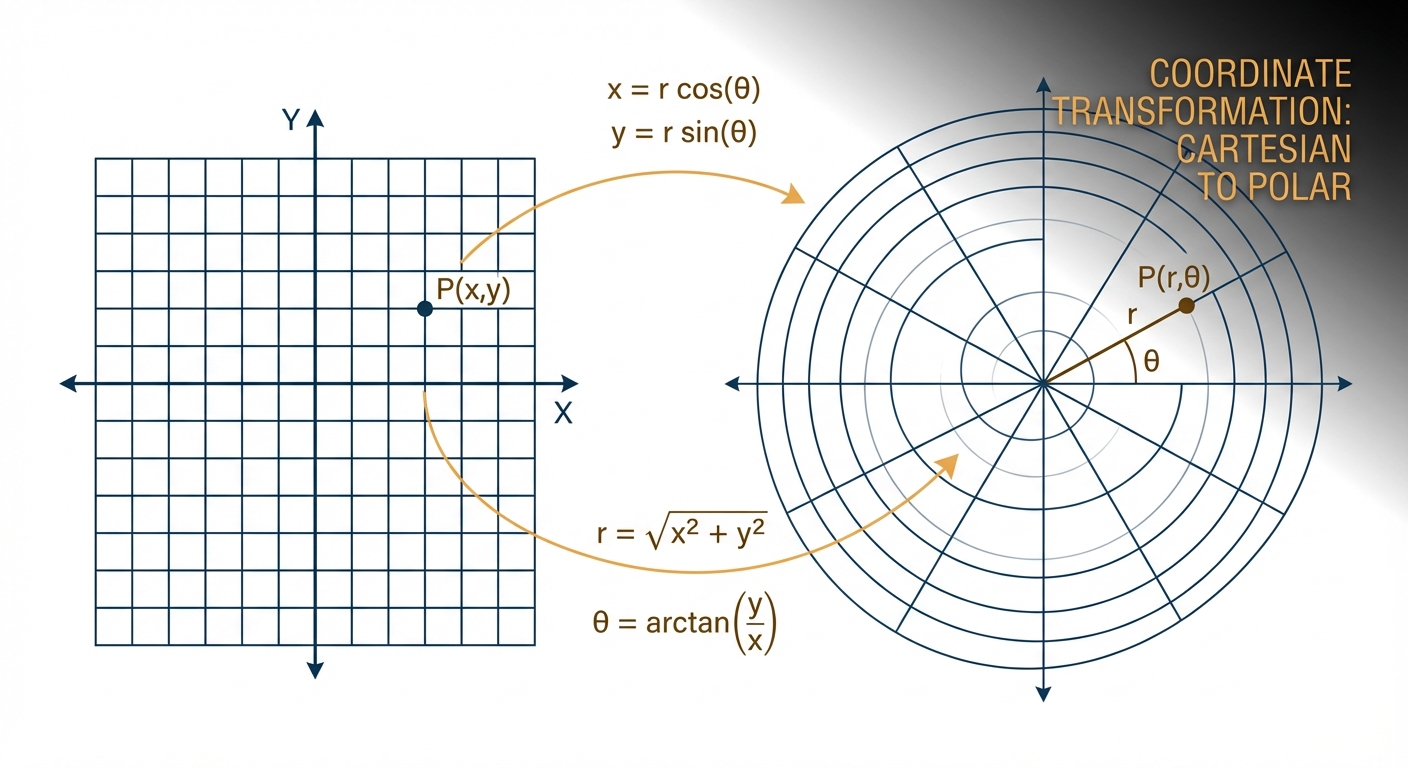
QJL: The 1-Bit Error Checker That Makes It Lossless
PolarQuant does the heavy lifting. It is responsible for the bulk of the compression. But no compression is perfect, and PolarQuant leaves behind a tiny residual error. This is where the second component comes in, and it is arguably just as clever.
The Quantised Johnson-Lindenstrauss (QJL) algorithm takes the small error left over from PolarQuant and squashes it down to a single sign bit per value: +1 or -1. That is it. One bit. The technique is based on the Johnson-Lindenstrauss lemma, a foundational result in dimensionality reduction that says you can project high-dimensional data into a much lower-dimensional space whilst preserving the distances between points.
What QJL does specifically is eliminate bias in the inner product estimation. This is critical because attention scores in transformers are computed as inner products (dot products) between query and key vectors. If your compression introduces a systematic bias in these dot products, the model’s attention mechanism starts paying attention to the wrong things. It is like having a compass that is consistently off by 3 degrees; every direction you follow drifts further from where you actually want to go.
QJL uses a special estimator that balances a high-precision query vector against the low-precision compressed data. The result is an unbiased inner product estimate with zero memory overhead. The 1-bit correction is so small it is essentially free to store, but it perfectly cancels out the residual error from PolarQuant.
// Stage 1: PolarQuant (main compression)
// 16-bit KV cache -> ~3 bits per channel
// Does most of the heavy lifting
// Tiny residual error remains

// Stage 2: QJL (error correction)
// Takes the residual from PolarQuant
// Reduces it to 1 sign bit (+1 or -1) per value
// Eliminates bias in attention score computation
// Memory overhead: essentially zero

// Combined: TurboQuant
// 3-bit KV cache with ZERO accuracy loss
// No retraining, no fine-tuning, no calibration
// Just swap it in and the model stays identical
Together, PolarQuant + QJL = TurboQuant. The compression engine and its error checker. The paper proves that TurboQuant achieves distortion rates within a factor of approximately 2.7 of the information-theoretic lower bound, the absolute mathematical limit of how well any quantiser could ever perform. In the language of information theory, this is approaching the Shannon limit. There is not much room left to improve.
“We also provide a formal proof of the information-theoretic lower bounds on best achievable distortion rate by any vector quantizer, demonstrating that TurboQuant closely matches these bounds, differing only by a small constant (approx 2.7) factor.” — Zandieh et al., TurboQuant: Online Vector Quantization with Near-optimal Distortion Rate, arXiv:2504.19874
The Numbers: What TurboQuant Actually Delivers
Theory is nice, but what actually happened when they tested this on real hardware with real models? Google ran TurboQuant through a gauntlet of benchmarks on open-source models (Gemma, Mistral, Llama) running on NVIDIA H100 GPUs. The results are not incremental. They are a step change.
The Headline Numbers
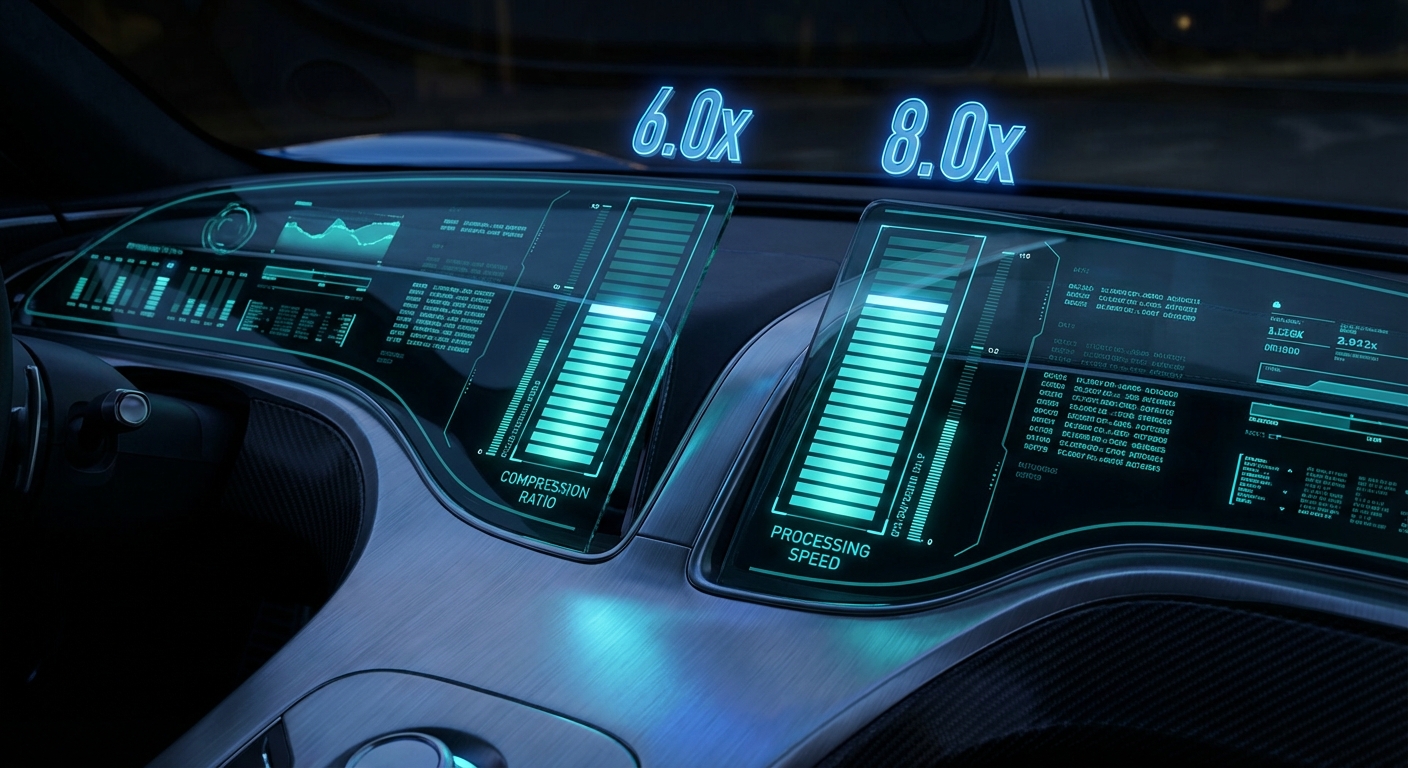
- 6x KV cache memory reduction. A cache that previously required 16 bits per value now needs under 3 bits. On a model that was using 6 GB of KV cache memory, you now need roughly 1 GB.
- Up to 8x attention speedup. The attention computation (the most expensive part of inference) runs up to 8 times faster on H100 GPUs. This does not mean the entire model is 8x faster, but the bottleneck operation is.
- Zero accuracy loss. At 3.5 bits per channel, TurboQuant achieves what the authors call “absolute quality neutrality.” The compressed model produces identical results to the uncompressed model. Even at 2.5 bits per channel, degradation is marginal.
- No retraining required. This is not a new model architecture. There is no fine-tuning step, no calibration dataset, no model-specific tuning. You slot TurboQuant into the inference pipeline and the existing model just works better.
Benchmark Breakdown
The team tested across five major long-context benchmarks:
- LongBench — question answering, summarisation, code generation across diverse tasks
- Needle in a Haystack — finding one specific piece of information buried in massive documents
- ZeroSCROLLS — long-document understanding tasks
- RULER — synthetic benchmarks that stress-test context window utilisation
- L-Eval — comprehensive evaluation of long-context capabilities
Across all of them, TurboQuant achieved perfect downstream results whilst reducing KV cache memory by at least 6x. PolarQuant alone was nearly lossless. With QJL added on top, it became mathematically unbiased.
The Stock Market Bloodbath (And Why Analysts Say Calm Down)
Google published TurboQuant on 24 March 2026. Within 48 hours, billions of dollars had been wiped off memory chip stocks across three continents.
The logic seemed straightforward: if AI models need 6x less memory, companies that make memory chips are going to sell fewer chips. Right?
The Damage Report
- SK Hynix (South Korea) — down 6.23%
- Samsung (South Korea) — down nearly 5%
- Kioxia (Japan) — down nearly 6%
- Micron (USA) — down over 20% across six trading sessions
- SanDisk (USA) — down 11%
- Western Digital (USA) — down 6.7%
- Seagate (USA) — down 8.5%
The broader Korean KOSPI index fell as much as 3%. Matthew Prince, CEO of Cloudflare, called it “Google’s DeepSeek moment,” referencing the January 2025 DeepSeek sell-off that wiped nearly a trillion dollars off the Nasdaq.
But here is the thing. Analysts are not panicking. In fact, most of them are telling investors to buy the dip.
Ray Wang, a memory analyst at SemiAnalysis, told CNBC:
“When you address a bottleneck, you are going to help AI hardware to be more capable. And the training model will be more powerful in the future. When the model becomes more powerful, you require better hardware to support it.” — Ray Wang, SemiAnalysis, via CNBC (March 2026)
Ben Barringer, head of technology research at Quilter Cheviot, was even more direct: “Memory stocks have had a very strong run and this is a highly cyclical sector, so investors were already looking for reasons to take profit. The Google Turboquant innovation has added to the pressure, but this is evolutionary, not revolutionary. It does not alter the industry’s long-term demand picture.”
For context, memory stocks had been on an absolute tear before this. Samsung was up nearly 200% over the prior year. SK Hynix and Micron were up over 300%. A correction was arguably overdue, and TurboQuant gave skittish investors the excuse they needed.
Jevons Paradox: Why Efficiency Makes You Use More, Not Less
The most important framework for understanding TurboQuant’s long-term impact is not computer science. It is economics. Specifically, a concept from 1865.
In The Coal Question, economist William Stanley Jevons documented something counterintuitive: when James Watt’s innovations made steam engines dramatically more fuel-efficient, Britain’s coal consumption did not fall. It increased tenfold. The efficiency gains lowered coal’s effective cost, which made it economical for new applications and industries. The per-unit savings were overwhelmed by the explosion in total usage.
This is the Jevons paradox, and it has been playing out in AI with striking precision. Between late 2022 and 2025, the cost of running large language models collapsed roughly a thousandfold. GPT-4-equivalent performance dropped from $20 to $0.40 per million tokens. Did people use fewer tokens? Enterprise generative AI spending skyrocketed from $11.5 billion in 2024 to $37 billion in 2025, a 320% increase. When OpenAI dropped API prices by 10x, API calls grew 100x.
The same pattern will almost certainly play out with TurboQuant. If it suddenly costs half as much to run a Frontier model, companies will not pocket the savings and go home. They will run bigger models, longer contexts, more agents, more concurrent sessions. Workloads that were previously too expensive become viable. The 200K-context analysis that cost too much to justify? Now it makes business sense. The always-on AI assistant that was too expensive to run 24/7? Now it is affordable.
Morgan Stanley’s analysts made exactly this argument, citing Jevons paradox to characterise the long-term impact on storage demand as “neutral to positive.” The market overpriced the short-term headline and underpriced the second-order effects.
What This Means for Anyone Using AI Right Now
Let us get concrete about who benefits and how.
Enterprises Running Models at Scale
If you are an enterprise running large language models in production, TurboQuant translates roughly to a 50% reduction in inference costs. This is not a marginal optimisation. This applies to every prompt, every API call, every chatbot response, every agentic workflow. API calls get cheaper. Faster responses. More requests per second on the same hardware. The ability to run longer context windows without hitting memory limits.
Context Windows Get Bigger on the Same Hardware
If a GPU was maxing out at a certain context length because the KV cache filled the available memory, TurboQuant effectively multiplies the available context by 6x. A model that topped out at 32K tokens on a given GPU could now handle 192K tokens. This is significant for code analysis, legal document review, medical record processing, and any workload where more context means better output.
The Anthropic Mythos Situation
Anthropic’s upcoming Mythos model has been described as “very expensive for us to serve, and will be very expensive for our customers to use.” Early pricing estimates suggest 2-5x the cost of Claude Opus. TurboQuant could meaningfully change that calculus. If inference costs drop by half, a model that was borderline unviable for production use cases suddenly becomes economically defensible. Whether Anthropic adopts TurboQuant specifically or implements similar techniques, the pressure to do so just became enormous.
Individual Power Users
Andrej Karpathy, former Tesla AI lead and OpenAI researcher, recently said in an interview that he gets “nervous when I have subscription left over” because “that just means I haven’t maximised my token throughput.” He now runs multiple AI agents in parallel across separate repository branches, treating token consumption as his primary productivity constraint. NVIDIA CEO Jensen Huang has said he expects employees earning $500,000 to use $250,000 worth of tokens. If TurboQuant halves the cost of those tokens, the effective value of every subscription doubles overnight.
Google’s Quiet Giant Move: Why They Published Instead of Hoarding
There is a pattern here that deserves attention. In 2017, a team at Google published “Attention Is All You Need” by Vaswani et al., the paper that introduced the transformer architecture. That single paper became the foundation for GPT, Claude, Gemini, Llama, Mistral, and essentially every large language model in existence. Most of Google’s competitors are built on Google’s published research.
They did it again with TurboQuant. Google could have kept this internal. They could have quietly deployed it across their infrastructure, pocketed the 50% cost savings on Gemini inference, and used the competitive advantage to undercut everyone else on pricing. That is the standard playbook. But they published it. The paper is on arXiv. The blog post explains the technique in detail. Community implementations appeared on PyPI and GitHub within days.
This is not altruism (Google benefits enormously from being the company that publishes foundational research, and they have the infrastructure to move fastest on their own inventions). But the effect is real. Every company running AI models, every open-source project, every independent developer benefits from this work being public.
As Martin Kleppmann writes in Designing Data-Intensive Applications, the most impactful systems are often the ones that reduce the cost of doing something by an order of magnitude, because they do not just make existing use cases cheaper; they create entirely new categories of application that were previously uneconomical. TurboQuant is precisely that kind of step change.
When TurboQuant Does Not Apply (The Honest Bit)
No article from this site would be credible without the caveats section, so here they are:
Case 1: Training Is Untouched
TurboQuant is an inference optimisation. It compresses the KV cache, which is used during inference (when the model generates responses). It does not reduce the cost of training a model. The multi-billion-dollar GPU clusters that companies like Google, OpenAI, and Meta use to train Frontier models are not affected. Training has its own bottlenecks (gradient accumulation, all-reduce communication, activation memory), and TurboQuant addresses none of them.
Case 2: It Only Compresses the KV Cache
The 6x memory reduction applies specifically to the KV cache, not to the model weights, not to the activations, and not to the total GPU memory usage. For many inference workloads, the KV cache is the dominant memory consumer, especially at long context lengths. But for short prompts on large models, the model weights themselves might be the bottleneck. TurboQuant helps a lot in the first scenario and less in the second.
Case 3: You Still Need GPUs
TurboQuant makes existing hardware more efficient. It does not eliminate the need for GPUs (or TPUs). You still need compute to run models. What changes is how much work each GPU can do. Think of it as improving fuel efficiency in a car: you still need the car, and you still need fuel, but you go further on each tank.
Case 4: The 8x Speedup Is for Attention, Not End-to-End
The headline “8x speedup” refers to the attention computation specifically, not the total inference time. A full model forward pass includes many other operations (feedforward layers, layer norms, embedding lookups). The end-to-end speedup depends on what fraction of total inference time is spent on attention. For long-context workloads, it is a large fraction. For short prompts, less so.
How This Actually Gets Deployed
One of TurboQuant’s strongest properties is how easy it is to adopt. Unlike techniques that require retraining or fine-tuning, TurboQuant is data-oblivious: it works without any dataset-specific preprocessing. The deployment path looks like:
- No model changes. The model weights, architecture, and training are all untouched. TurboQuant operates entirely at the inference layer.
- Swap the KV cache quantiser. Replace the existing KV cache storage with TurboQuant’s polar coordinate quantisation. This is a software change in the inference engine.
- Choose your bit-width. At 3.5 bits per channel, you get zero accuracy loss. At 2.5 bits per channel, you get even more compression with marginal degradation. Pick based on your quality requirements.
- Deploy. Run the same prompts, get the same results, use 6x less KV cache memory, and compute attention up to 8x faster.
Community implementations have already appeared. A pip-installable turboquant package is on PyPI. Third-party implementations in MLX (for Apple Silicon) and Triton (for custom GPU kernels) were published within days of the announcement. The official Google code is expected in Q2 2026.
# Community implementation (illustrative)
# pip install turboquant
from turboquant import TurboQuantConfig, apply_turboquant

config = TurboQuantConfig(
    bits_per_channel=3.5,   # Zero accuracy loss
    enable_qjl=True,        # Error correction stage
)

# Apply to any HuggingFace model's KV cache
model = apply_turboquant(model, config)

# Inference runs as normal -- same API, same outputs
# But KV cache is now 6x smaller and attention is up to 8x faster
output = model.generate(input_ids, max_new_tokens=512)
What to Check Right Now
- Audit your KV cache memory usage. If you are running models in production, profile how much GPU memory your KV cache consumes. If it is a significant fraction of total memory (common for long-context workloads), TurboQuant could give you an immediate and substantial improvement.
- Watch for framework integration. Keep an eye on vLLM, TensorRT-LLM, and HuggingFace TGI for native TurboQuant support. Once it lands in these frameworks, adoption becomes a config flag.
- Re-evaluate your context length limits. If you capped context length because of memory constraints, TurboQuant may let you lift those caps on existing hardware. Longer context often means better output quality.
- Read the actual paper. The TurboQuant paper (arXiv:2504.19874) and the PolarQuant paper (arXiv:2502.02617) are both well-written and surprisingly accessible. The Google Research blog post is an excellent entry point if you want the intuition without the proofs.
- Don’t panic-sell memory stocks based on headlines. The Jevons paradox has held true for every major compute efficiency improvement in history. Efficiency does not reduce demand; it creates it. The analysts calling this “evolutionary, not revolutionary” for the memory industry are probably right.
- Try it yourself. The community turboquant PyPI package and the turboquant-pytorch GitHub repo let you test it on your own models today.
Video Attribution
This article was inspired by Wes Roth’s excellent breakdown of TurboQuant. Watch the full video below:
nJoy 😉