Category: AI Foundations

In the previous article on context management, we built the machinery by hand: sliding windows, compaction, PostgreSQL-backed memory stores, A2A handoffs. That is genuinely useful knowledge. But at some point you look at the boilerplate and think: surely someone has already solved the plumbing. They have. It is called Letta, it is open source, and it implements every pattern we discussed as a first-class runtime. This article is about how to actually use it, with Node.js, in a way that is production-shaped rather than tutorial-shaped.

What Letta Is (and What It Is Not)

Letta is the production evolution of MemGPT, a research project from UC Berkeley that demonstrated you could give an LLM the ability to manage its own memory through tool calls, effectively creating unbounded context. The research paper was elegant; the original codebase was academic. Letta is the commercial rewrite: a stateful agent server with a proper REST API, a TypeScript/Node.js client, PostgreSQL-backed persistence, and a web-based Agent Development Environment (ADE) at app.letta.com.

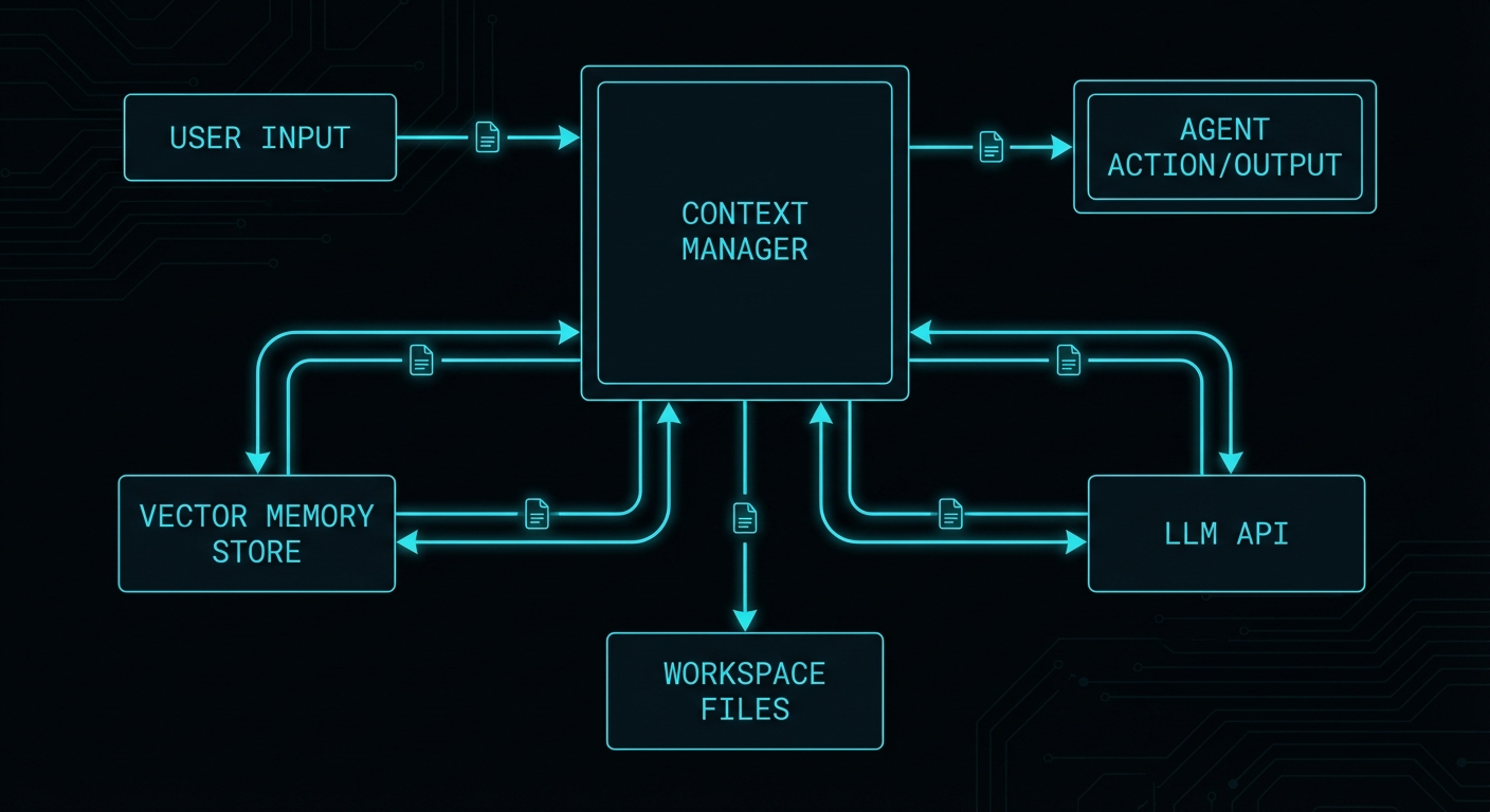
The key architectural commitment Letta makes is that the server owns all state. You do not manage a message array in your application. You do not serialise session state to disk. You do not build a compaction loop. You send a new user message, the Letta server handles the rest: it injects the right memory blocks, runs the agent, manages the context window, persists everything to its internal PostgreSQL database, and returns the response. Your application is stateless; Letta’s server is stateful. This is Kleppmann’s stream processing model applied to agents: the server is the durable log, and your application is just a producer/consumer.

What Letta is not: a model provider, a prompt engineering framework, or a replacement for your orchestration logic when you need bespoke control. It is an agent runtime. You still choose the model (any OpenAI-compatible endpoint, Anthropic, Ollama, etc.). You still design the tools. You still decide the architecture. Letta manages context, memory, and persistence so you do not have to.

Running Letta: Docker in Two Minutes

The fastest path to a running Letta server is Docker. One command, PostgreSQL included:

docker run \
  -v ~/.letta/.persist/pgdata:/var/lib/postgresql/data \
  -p 8283:8283 \
  -e OPENAI_API_KEY="sk-..." \
  -e ANTHROPIC_API_KEY="sk-ant-..." \
  letta/letta:latest

The server starts on port 8283. Agent data persists to the mounted volume. The ADE at https://app.letta.com can connect to your local instance for visual inspection and debugging. Point it at http://localhost:8283 and you have a full development environment with memory block viewers, message history, and tool call traces.

For production, you will want to externalise the PostgreSQL instance (a managed RDS or Cloud SQL instance), set LETTA_PG_URI to point at it, and run Letta behind a reverse proxy with TLS. The Letta server itself is stateless between requests; it is the database that holds everything. That means you can run multiple Letta instances behind a load balancer pointing at the same PostgreSQL, which is the correct horizontal scaling pattern.

Install the Node.js client:

npm install @letta-ai/letta-client

Connect to your local or remote server:

import Letta from '@letta-ai/letta-client';

// Local development
const client = new Letta({ baseURL: 'http://localhost:8283' });

// Letta Cloud (managed, no self-hosting required)
const client = new Letta({ apiKey: process.env.LETTA_API_KEY });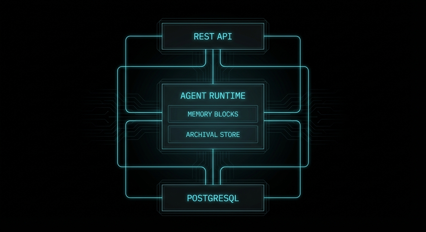

Memory Blocks: The Core Abstraction

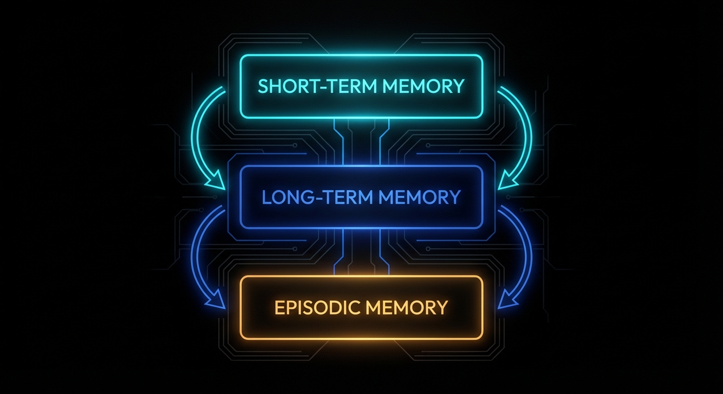
If you read the context management article, you encountered the concept of “always-in-context pinned memory”: facts that never get evicted, always present at the top of the system prompt. Letta formalises this as memory blocks. A memory block is a named, bounded string that gets prepended to the agent’s system prompt on every single turn, in a structured XML-like format the model can read and modify.

This is what the model actually sees in its context window:

<memory_blocks>

<persona>
<description>Stores details about your persona, guiding how you behave.</description>
<metadata>chars_current=128 | chars_limit=5000</metadata>
<value>I am Sam, a persistent assistant that remembers across sessions.</value>
</persona>

<human>
<description>Key details about the person you're conversing with.</description>
<metadata>chars_current=84 | chars_limit=5000</metadata>
<value>Name: Alice. Role: senior backend engineer. Prefers concise answers. Uses Node.js.</value>
</human>

</memory_blocks>

Three things make this powerful. First, the model can see the character count and limit, so it manages the block like a finite buffer rather than writing without restraint. Second, the description field is the primary signal the model uses to decide how to use each block: write a bad description and the agent will misuse it. Third, blocks are editable by the agent via built-in tools: when the agent learns something worth preserving, it calls core_memory_replace or core_memory_append, and that change is persisted immediately to the database and visible on the next turn.

Here is a full agent creation with custom memory blocks in Node.js:

// create-agent.js
import Letta from '@letta-ai/letta-client';

const client = new Letta({ baseURL: 'http://localhost:8283' });

const agent = await client.agents.create({
  name: 'dev-assistant',
  model: 'anthropic/claude-3-7-sonnet-20250219',
  embedding: 'openai/text-embedding-3-small', // required for archival memory search
  memory_blocks: [
    {
      label: 'persona',
      value: 'I am a persistent dev assistant. I remember what you are working on, your preferences, and your past decisions. I am direct and do not pad answers.',
      limit: 5000,
    },
    {
      label: 'human',
      value: '', // starts empty; agent fills this in as it learns about the user
      limit: 5000,
    },
    {
      label: 'project',
      description: 'The current project the user is working on: name, stack, key decisions, and open questions. Update whenever the project context changes.',
      value: '',
      limit: 8000,
    },
    {
      label: 'mistakes',
      description: 'A log of mistakes or misunderstandings from past conversations. Consult this before making similar suggestions. Add to it when corrected.',
      value: '',
      limit: 3000,
    },
  ],
});

console.log('Agent created:', agent.id);
// Save this ID — it is the persistent identifier for this agent across all sessions

The project and mistakes blocks are custom: Letta does not know what they are for, but the model does, because you told it in the description field. This is where Hofstadter’s recursion shows up in the most practical way: you are configuring an agent’s memory by describing to the agent what memory is for, and the agent then self-organises accordingly.

Sending Messages: The Stateless Caller Pattern

This is the part that trips up developers coming from a hand-rolled context manager. With Letta, you do not maintain a message array. You do not pass the conversation history. You send only the new message. The server knows the history:

// chat.js
import Letta from '@letta-ai/letta-client';

const client = new Letta({ baseURL: 'http://localhost:8283' });

async function chat(agentId, userMessage) {
  const response = await client.agents.messages.create(agentId, {
    messages: [
      { role: 'user', content: userMessage },
    ],
  });

  // Extract the final text response from the run steps
  const textResponse = response.messages
    .filter(m => m.message_type === 'assistant_message')
    .map(m => m.content)
    .join('\n');

  return textResponse;
}

// First message: the agent starts learning about the user
const reply1 = await chat('agent-id-here', 'Hi, I\'m working on a Node.js API that serves a mobile app. Postgres for data, Redis for sessions.');
console.log(reply1);

// Second message, completely separate process invocation:
// The agent already knows everything from the first message.
const reply2 = await chat('agent-id-here', 'What database am I using again?');
console.log(reply2); // → "You're using Postgres for data and Redis for sessions."

The agent’s memory block for project was updated by the model itself during the first turn via its built-in memory tools. On the second turn, that block is injected back into context automatically. Your application code never touched any of it.

You can inspect what the agent currently knows at any point via the API:

// Peek at the agent's current memory state
const projectBlock = await client.agents.blocks.retrieve(agentId, 'project');
console.log('What the agent knows about your project:');
console.log(projectBlock.value);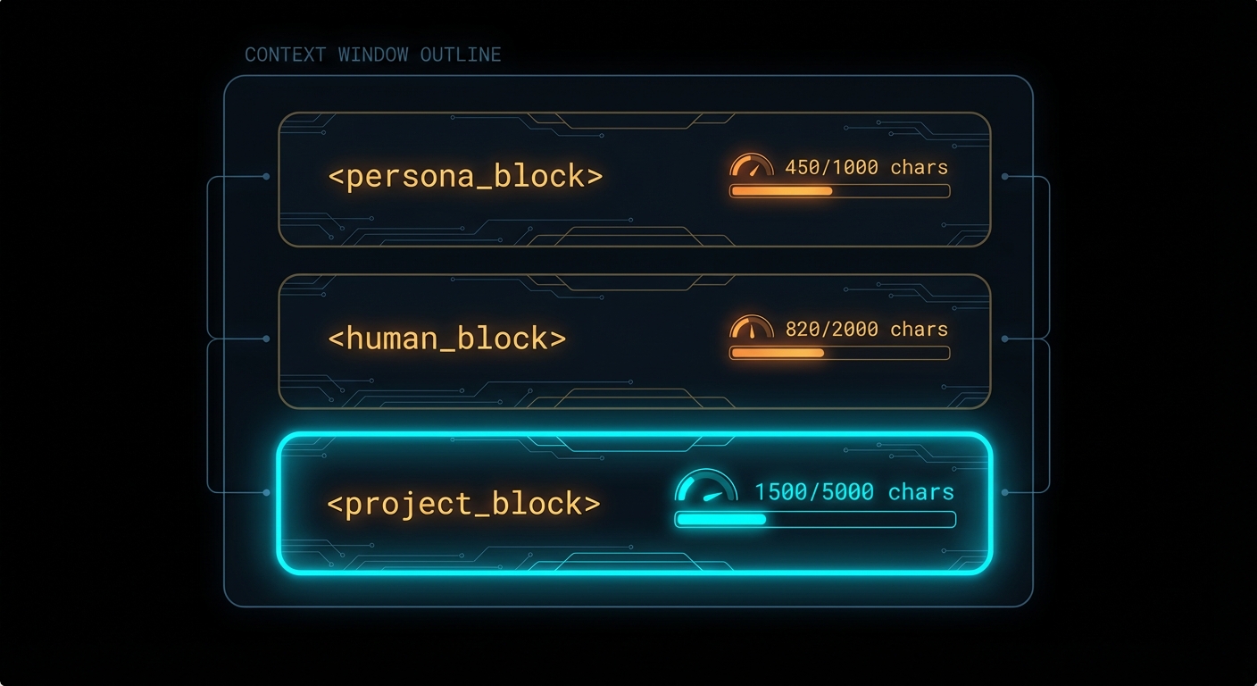

Archival Memory: The Infinite Store

Memory blocks are bounded (5,000 characters by default). For anything that does not fit, Letta provides archival memory: an external vector store backed by pgvector (in the self-hosted setup) or Letta Cloud’s managed index. The agent accesses it via two built-in tool calls that appear in its context as available tools: archival_memory_insert and archival_memory_search.

You do not have to configure these tools; they are always present. When the agent encounters a piece of information that is too large or too ephemeral for a core memory block, it decides to archive it. When it needs to recall something from the past, it issues a semantic search. All of this is embedded in the agent’s reasoning loop, not your application code.

You can also write to archival memory programmatically from your application, which is useful for seeding an agent with existing knowledge:

// seed-archival-memory.js
// Useful for bulk-loading documentation, past conversation summaries,
// or domain knowledge before the agent starts interacting with users

async function seedKnowledge(agentId, documents) {
  for (const doc of documents) {
    await client.agents.archivalMemory.create(agentId, {
      text: doc.content,
    });
    console.log(`Seeded: ${doc.title}`);
  }
}

// Example: seed with codebase context
await seedKnowledge(agentId, [
  { title: 'Auth module', content: 'The authentication module uses JWT with 24h expiry. Refresh tokens stored in Redis with 30-day TTL. See src/auth/...' },
  { title: 'DB schema', content: 'Main tables: users, sessions, events. users.id is UUID. events has a JSONB payload column...' },
  { title: 'Deployment', content: 'Production runs on Render. Two services: api (Node.js) and worker (Bull queue). Shared Postgres on Supabase...' },
]);

// Search archival memory (what the agent would do internally)
const results = await client.agents.archivalMemory.list(agentId, {
  query: 'authentication refresh token',
  limit: 5,
});

Multi-Agent Patterns with Shared Memory Blocks

This is where Letta’s design diverges most sharply from a DIY approach. In our context management article, the A2A section covered how to pass context between agents via structured handoff payloads. Letta adds a second mechanism that is often cleaner: shared memory blocks. A block attached to multiple agents is simultaneously visible to all of them. When any agent updates it, all agents see the change on their next turn.

The coordination pattern this enables: a supervisor agent writes its plan to a shared task_state block. All worker agents have that block in their context windows. The supervisor does not need to message each worker explicitly; the workers read the shared state and self-coordinate. This is closer to a shared blackboard than a message bus, and for many use cases it is significantly simpler:

// multi-agent-setup.js
import Letta from '@letta-ai/letta-client';

const client = new Letta({ baseURL: 'http://localhost:8283' });

// Create a shared state block
const taskStateBlock = await client.blocks.create({
  label: 'task_state',
  description: 'Current task status shared across all agents. Supervisor writes the plan and tracks progress. Workers read their assignments and update status when done.',
  value: JSON.stringify({ status: 'idle', tasks: [], results: [] }),
  limit: 10000,
});

// Create supervisor agent
const supervisor = await client.agents.create({
  name: 'supervisor',
  model: 'anthropic/claude-3-7-sonnet-20250219',
  memory_blocks: [
    { label: 'persona', value: 'I coordinate teams of specialist agents. I decompose tasks, assign them, and synthesise results.' },
  ],
  block_ids: [taskStateBlock.id], // attach shared block
});

// Create worker agents — all share the same task state block
const workers = await Promise.all(['code-analyst', 'security-reviewer', 'doc-writer'].map(name =>
  client.agents.create({
    name,
    model: 'anthropic/claude-3-5-haiku-20241022', // cheaper model for workers
    memory_blocks: [
      { label: 'persona', value: `I am a specialist ${name} agent. I read my assignments from task_state and write my results back.` },
    ],
    block_ids: [taskStateBlock.id],
    tags: ['worker'], // tags enable broadcast messaging
  })
));

For direct agent-to-agent messaging, Letta provides three built-in tools the model can call: send_message_to_agent_async (fire-and-forget, good for kicking off background work), send_message_to_agent_and_wait_for_reply (synchronous, good for gathering results), and send_message_to_agents_matching_all_tags (broadcast to a tagged group).

The supervisor-worker pattern with broadcast looks like this from the application perspective:

// Run the supervisor with a task; it handles delegation internally
const result = await client.agents.messages.create(supervisor.id, {
  messages: [{
    role: 'user',
    content: 'Review the PR at github.com/org/repo/pull/42. Get security, code quality, and docs perspectives.',
  }],
});

// The supervisor will internally:
// 1. Decompose the task into three sub-tasks
// 2. Call send_message_to_agents_matching_all_tags({ tags: ['worker'], message: '...' })
// 3. Each worker agent processes its sub-task
// 4. Results flow back to the supervisor
// 5. Supervisor synthesises and responds to the original message

// You can watch the shared block update in real time:
const state = await client.blocks.retrieve(taskStateBlock.id);
console.log(JSON.parse(state.value));

Conversations API: One Agent, Many Users

The multi-user pattern in Letta has two flavours. The simpler one: create one agent per user. Each agent has its own memory blocks and history. Clean isolation, straightforward. The more powerful one, added in early 2026: the Conversations API, which lets multiple users message a single agent through independent conversation threads without sharing message history.

This is the right pattern for a shared assistant that should have a consistent persona and knowledge base across all users, while keeping each user’s conversation private:

// conversations.js

// Create a single shared agent (one-time setup)
const sharedAssistant = await client.agents.create({
  name: 'company-assistant',
  model: 'anthropic/claude-3-7-sonnet-20250219',
  memory_blocks: [
    {
      label: 'persona',
      value: 'I am the Acme Corp internal assistant. I know our products, policies, and engineering practices.',
    },
    {
      label: 'policies',
      description: 'Company policies. Read-only. Do not modify.',
      value: 'Data retention: 90 days. Escalation path: ops → engineering → CTO. ...',
      read_only: true,
    },
  ],
});

// Each user gets their own conversation thread with this agent
async function getUserConversation(agentId, userId) {
  // List existing conversations for this user
  const conversations = await client.agents.conversations.list(agentId, {
    user_id: userId,
  });

  if (conversations.length > 0) {
    return conversations[0].id; // resume existing
  }

  // Create a new conversation thread for this user
  const conversation = await client.agents.conversations.create(agentId, {
    user_id: userId,
  });
  return conversation.id;
}

// Send a message within a user's private conversation thread
async function sendMessage(agentId, conversationId, userMessage) {
  return client.agents.messages.create(agentId, {
    conversation_id: conversationId,
    messages: [{ role: 'user', content: userMessage }],
  });
}

// Usage: two users, one agent, completely isolated message histories
const aliceConvId = await getUserConversation(sharedAssistant.id, 'user-alice');
const bobConvId   = await getUserConversation(sharedAssistant.id, 'user-bob');

await sendMessage(sharedAssistant.id, aliceConvId, 'What is our data retention policy?');
await sendMessage(sharedAssistant.id, bobConvId,   'How do I escalate a prod incident?');

Connecting to What We Built Before

If you built the context manager from the previous article, you already understand what Letta is doing under the hood. The memory blocks are the workspace injection layer (SOUL.md, USER.md, etc.) made into a first-class API. The built-in memory tools are the memoryFlush hook, made automatic. The Conversations API is the session store with user-scoped RLS, managed for you. The archival memory tools are the PostgresMemoryStore with pgvector, managed for you.

The practical question is when to use Letta versus building your own. The answer is usually: use Letta when the standard patterns fit, build your own when they do not. Letta is excellent for: persistent user-facing assistants, multi-agent systems with shared state, anything where you need reliable memory across sessions without owning the infrastructure. Build your own when: you need sub-millisecond latency and cannot afford the Letta server round-trip, you need extreme control over what enters the context window, or you are building a very specialised agent loop that does not match any of Letta’s patterns.

You can also combine both: use Letta for its memory management while driving the agent loop from your own orchestration code. Create the agent via Letta’s API, send messages via the SDK, but handle tool routing, A2A handoffs, and business logic in your application layer:

// hybrid-orchestrator.js
// Use Letta for memory; own your tool routing

import Letta from '@letta-ai/letta-client';
import { handleA2AHandoff } from './a2a-context-bridge.js';
import { handleDomainTool } from './domain-tools.js';

const client = new Letta({ baseURL: 'http://localhost:8283' });

async function runTurn(agentId, userMessage, userId) {
  const response = await client.agents.messages.create(agentId, {
    messages: [{ role: 'user', content: userMessage }],
    // Inject user ID as context so the agent can reference who it's talking to
    stream_steps: false,
  });

  // Process any tool calls that need external routing
  for (const step of response.messages) {
    if (step.message_type === 'tool_call' && step.tool_name === 'delegate_to_agent') {
      // Route A2A handoffs through our own bridge
      const handoffResult = await handleA2AHandoff(step.tool_arguments, userId);

      // Inject the result back into the agent's context as a tool result
      await client.agents.messages.create(agentId, {
        messages: [{
          role: 'tool',
          content: JSON.stringify(handoffResult),
          tool_call_id: step.tool_call_id,
        }],
      });
    }

    if (step.message_type === 'tool_call' && step.tool_name.startsWith('domain_')) {
      const result = await handleDomainTool(step.tool_name, step.tool_arguments);
      await client.agents.messages.create(agentId, {
        messages: [{
          role: 'tool',
          content: JSON.stringify(result),
          tool_call_id: step.tool_call_id,
        }],
      });
    }
  }

  return response.messages
    .filter(m => m.message_type === 'assistant_message')
    .map(m => m.content)
    .join('\n');
}

Deploying Custom Tools

Letta supports three tool types. Server-side tools have code that runs inside the Letta server’s sandboxed environment: safe for untrusted logic, limited in what they can access. MCP tools connect to any Model Context Protocol server: your agent can use any tool exposed by an MCP-compatible service (file systems, databases, web browsers, code execution). Client-side tools return only the JSON schema to the model; your application handles execution and passes the result back.

For production integrations, client-side tools are usually the right choice: your application owns the execution environment, credentials, and error handling. Register the schema with Letta so the model knows the tool exists; intercept the tool call in your application code:

// register-tools.js

// Register a client-side tool (schema only — you handle execution)
const dbQueryTool = await client.tools.create({
  name: 'query_database',
  description: 'Execute a read-only SQL query against the application database. Use for looking up user data, orders, or product information.',
  tags: ['database', 'read-only'],
  source_type: 'json', // client-side: no code, just schema
  json_schema: {
    name: 'query_database',
    description: 'Execute a read-only SQL query',
    parameters: {
      type: 'object',
      properties: {
        query: {
          type: 'string',
          description: 'The SQL query to run. SELECT only. No mutations.',
        },
        limit: {
          type: 'number',
          description: 'Maximum rows to return (default 20, max 100).',
        },
      },
      required: ['query'],
    },
  },
});

// Attach the tool to an agent
await client.agents.tools.attach(agentId, dbQueryTool.id);

What to Watch Out For

• The agent creates its own memory; don’t fight it. The model decides what goes into memory blocks and when. If the agent is not remembering something you expect it to, improve the description field on the relevant block. The description is the only instruction the model has for deciding when to write to that block.
• Block limits are character counts, not token counts. A 5,000-character block costs roughly 1,250 tokens in your context window on every turn. If you have six blocks at 5,000 chars each, you have already spent 7,500 tokens before a single message is processed. Be deliberate about how many blocks you create and how large they are.
• Shared blocks have last-write-wins semantics. If two agents update the same shared block concurrently, the last write overwrites the earlier one. For coordination state that multiple agents write, use a structured JSON format inside the block and have agents do read-modify-write operations carefully. Or use a dedicated supervisor agent as the sole writer.
• One agent per user is not always the right model. For a large user base, thousands of agents each with their own archival memory index can become expensive to manage. The Conversations API lets one agent serve many users without multiplying infrastructure; evaluate whether your use case actually needs per-user agents or just per-user conversation isolation.
• Seed archival memory before go-live. An agent with an empty archival store has no domain knowledge beyond its system prompt. Invest time before launch in bulk-loading your codebase context, documentation, past decision logs, or relevant domain content. A well-seeded archival store transforms a generic assistant into something that genuinely knows your system.
• Use Claude 3.5 Haiku or GPT-4o mini for worker agents in multi-agent systems. The frontier models (Claude 3.7 Sonnet, GPT-4o) are necessary for the supervisor that does planning and synthesis; they are overkill for workers executing narrow, well-defined tasks. The cost difference is roughly 10x; the capability difference for simple tasks is negligible.
• Heartbeats are the agent’s “thinking” loop. When a tool call returns request_heartbeat: true, Letta re-invokes the agent so it can reason about the result before responding. This is how multi-step reasoning works. Do not disable heartbeats on tasks that require chaining tool calls; you will get shallow, single-step responses.

nJoy 😉

At some point, every AI agent developer has the same moment of horror: the agent you carefully built, the one that was doing so well three hours into a session, suddenly starts asking what the project is called. It has forgotten. Not because the model is bad, but because you handed it a finite window and then silently watched it fill up. Context management is the unglamorous, absolutely load-bearing discipline that separates a demo agent from one that can actually work for eight hours straight. This article is about building the machinery that keeps agents sane over time, in Node.js, with reference to how production open-source systems like OpenClaw and Letta handle it.

The Problem Is Not the Model

Every large language model has a context window: a fixed maximum number of tokens it can process in a single forward pass. GPT-4o and GPT-4.5 sit at 128k tokens. Claude 3.7 Sonnet reaches 200k. Gemini 2.0 Flash and Gemini 1.5 Pro push to 1 million. DeepSeek-V3 and its reasoning sibling R1 offer 128k with strong cost-per-token economics. Those numbers sound enormous until you are running an agentic loop where each iteration appends tool call inputs, tool call outputs, file contents, and the model’s reasoning to the running transcript. A 128k window fills in roughly two to three hours of intensive agentic work. Gemini’s million-token window buys you longer headroom, but it does not buy you infinite headroom, and at scale the per-token cost of a full-context pass is not trivial. After that, you hit the wall.

It is also worth noting that extended thinking models like Claude 3.7 Sonnet with extended thinking enabled, or OpenAI’s o3, consume context faster than their base counterparts: the reasoning trace itself occupies tokens inside the window. A single extended-thinking turn on a hard problem can eat 10–20k tokens of reasoning before a single word of output is produced. Factor this into your compaction thresholds.

The naive response is to just truncate. Drop the oldest messages, keep the newest. This is the equivalent of giving someone severe anterograde amnesia: they can function in the immediate present, but every decision they make is disconnected from anything they learned more than ten minutes ago. For simple chatbots, this is acceptable. For agents executing multi-step plans across files, APIs, and codebases, it is a reliability catastrophe.

The sophisticated response, which is what this article covers, is to treat context as a managed resource: track it, compress it intelligently, extract durable knowledge before it falls off the edge, and retrieve relevant pieces back in when needed. Kleppmann’s framing in Designing Data-Intensive Applications applies here more than you might expect: the problem of context management is structurally identical to the problem of bounded buffers in streaming systems. You have a producer (the agent loop) generating data faster than the consumer (the context window) can hold it, and you need a backpressure strategy.

Three Memory Layers: Short, Long, and Episodic

Before writing any code, the mental model matters. Agentic memory systems have three distinct layers, each with different characteristics and different management strategies.

Short-term memory is the context window itself. Everything currently loaded into the model’s active attention. Fast, expensive per-token, bounded. This is where the current conversation, active tool results, and working state live. It is managed by controlling what gets added and what gets evicted.

Long-term memory is external storage: a vector database, a set of Markdown files, a SQL table. It is unbounded, cheap, and requires an explicit retrieval step to bring relevant pieces back into the context window when needed. This is where accumulated knowledge, user preferences, project facts, and prior decisions live.

Episodic memory is a specific log of past events: what happened at 14:32 on Tuesday, which tool calls were made, what the user said three sessions ago. It sits conceptually between the two: it is stored externally but is indexed by time and event rather than semantic content.

Production systems implement all three. OpenClaw, for instance, uses MEMORY.md for curated long-term facts and memory/YYYY-MM-DD.md files for episodic daily logs, with a vector search layer (SQLite + embeddings) providing semantic retrieval over both. Letta (formerly MemGPT) uses a tiered architecture with in-context “core memory” blocks and out-of-context “archival storage” accessed via tool calls. Different designs, same underlying problem decomposition.

Here is the baseline Node.js structure we will build on throughout this article:

// context-manager.js
export class ContextManager {
  constructor({ maxTokens = 100000, reserveTokens = 20000 } = {}) {
    this.maxTokens = maxTokens;
    this.reserveTokens = reserveTokens;
    this.messages = [];          // short-term: in-context history
    this.longTermMemory = [];    // long-term: persisted facts
    this.episodicLog = [];       // episodic: timestamped event log
  }

  get availableTokens() {
    return this.maxTokens - this.reserveTokens - this.estimateTokens(this.messages);
  }

  estimateTokens(messages) {
    // Rough heuristic: 1 token ≈ 4 characters
    const text = messages.map(m => m.content ?? JSON.stringify(m)).join('');
    return Math.ceil(text.length / 4);
  }

  addMessage(role, content) {
    this.messages.push({ role, content, timestamp: Date.now() });
    this.episodicLog.push({ role, content, timestamp: Date.now() });
  }

  getMessages() {
    return this.messages;
  }
}

Strategy 1: The Sliding Window

The sliding window is the simplest strategy and the right starting point. Keep only the most recent N tokens of conversation history. When the window fills, drop messages from the front. It has one job: prevent the context from overflowing. It does that job perfectly and remembers nothing else.

// sliding-window.js
import { ContextManager } from './context-manager.js';

export class SlidingWindowManager extends ContextManager {
  constructor(options) {
    super(options);
    this.systemPrompt = '';
  }

  setSystemPrompt(prompt) {
    this.systemPrompt = prompt;
  }

  addMessage(role, content) {
    super.addMessage(role, content);
    this.evict();
  }

  evict() {
    // Always keep the system prompt budget separate
    const systemTokens = Math.ceil(this.systemPrompt.length / 4);
    const budget = this.maxTokens - this.reserveTokens - systemTokens;

    while (this.estimateTokens(this.messages) > budget && this.messages.length > 1) {
      this.messages.shift(); // drop oldest
    }
  }

  buildPrompt() {
    return [
      { role: 'system', content: this.systemPrompt },
      ...this.messages,
    ];
  }
}

This is appropriate for stateless tasks: a customer support bot handling a single issue, a code review agent analysing one file, a single-turn tool call. It is not appropriate for anything that runs across multiple turns where prior context matters. The moment your agent needs to reference a decision it made fifteen minutes ago, the sliding window has already dropped it.

One refinement worth adding immediately: protect critical messages from eviction. System messages, task initialisation messages, and tool call summaries that represent completed milestones should be pinned. Everything else is fair game:

addMessage(role, content, { pinned = false } = {}) {
  this.messages.push({ role, content, timestamp: Date.now(), pinned });
  this.evict();
}

evict() {
  const systemTokens = Math.ceil(this.systemPrompt.length / 4);
  const budget = this.maxTokens - this.reserveTokens - systemTokens;

  // Only evict unpinned messages, oldest first
  while (this.estimateTokens(this.messages) > budget) {
    const evictIdx = this.messages.findIndex(m => !m.pinned);
    if (evictIdx === -1) break; // everything is pinned, cannot evict
    this.messages.splice(evictIdx, 1);
  }
}

Strategy 2: Compaction (Summarisation)

Compaction is sliding window with a conscience. Instead of silently dropping old messages, you first ask the model to summarise them into a compact representation, then replace the original messages with that summary. The agent retains a compressed understanding of what happened; it just loses the verbatim transcript.

This is the approach OpenClaw uses under the name “compaction.” When a session approaches the token limit (controlled by reserveTokens and keepRecentTokens config), the Gateway triggers a compaction: the older portion of the transcript is summarised into a single entry, pinned at the top of the history, and the raw messages are replaced. Critically, OpenClaw triggers a “memory flush” before compaction: a silent agentic turn that instructs the model to write any durable facts to the MEMORY.md file before the context is compressed. The insight here is important: compaction loses detail, so extract the durable bits to long-term storage first.

Here is a Node.js implementation:

// compacting-manager.js
import Anthropic from '@anthropic-ai/sdk';
import { ContextManager } from './context-manager.js';

const client = new Anthropic();

export class CompactingManager extends ContextManager {
  constructor(options) {
    super({
      maxTokens: 100000,
      reserveTokens: 16384,
      keepRecentTokens: 20000,
      ...options,
    });
    this.systemPrompt = '';
    this.compactionSummary = null; // the pinned summary entry
  }

  setSystemPrompt(prompt) {
    this.systemPrompt = prompt;
  }

  addMessage(role, content) {
    super.addMessage(role, content);
  }

  shouldCompact() {
    const used = this.estimateTokens(this.messages);
    const threshold = this.maxTokens - this.reserveTokens - this.keepRecentTokens;
    return used > threshold;
  }

  async compact() {
    if (this.messages.length < 4) return; // not enough to summarise

    // Split: keep the most recent messages verbatim, compact the rest
    const recentTokenTarget = this.keepRecentTokens;
    let recentTokens = 0;
    let splitIndex = this.messages.length;

    for (let i = this.messages.length - 1; i >= 0; i--) {
      const msgTokens = Math.ceil((this.messages[i].content?.length ?? 0) / 4);
      if (recentTokens + msgTokens > recentTokenTarget) {
        splitIndex = i + 1;
        break;
      }
      recentTokens += msgTokens;
    }

    const toCompact = this.messages.slice(0, splitIndex);
    const toKeep = this.messages.slice(splitIndex);

    if (toCompact.length === 0) return;

    console.log(`[CompactingManager] Compacting ${toCompact.length} messages into summary...`);

    const summaryText = await this.summarise(toCompact);

    // Replace compacted messages with the summary entry
    this.compactionSummary = {
      role: 'user',
      content: `[Compacted history summary]\n${summaryText}`,
      timestamp: Date.now(),
      pinned: true,
      isCompactionSummary: true,
    };

    this.messages = [this.compactionSummary, ...toKeep];
    console.log(`[CompactingManager] Done. Messages reduced to ${this.messages.length}.`);
  }

  async summarise(messages) {
    const transcript = messages
      .map(m => `${m.role.toUpperCase()}: ${m.content}`)
      .join('\n\n');

    const response = await client.messages.create({
      model: 'claude-3-5-haiku-20241022', // use a fast, cheap model for compaction — not your main model
      max_tokens: 2048,
      messages: [
        {
          role: 'user',
          content: `Summarise the following conversation history. Preserve:
- All decisions made and their reasoning
- Tasks completed and their outcomes
- Any errors encountered and how they were resolved
- Important facts, file names, IDs, or values that may be needed later
- The current state of any ongoing work

Be concise but complete. Use bullet points.

CONVERSATION:
${transcript}`,
        },
      ],
    });

    return response.content[0].text;
  }

  async addMessageAndMaybeCompact(role, content) {
    this.addMessage(role, content);
    if (this.shouldCompact()) {
      await this.memoryFlush(); // extract durable facts first
      await this.compact();
    }
  }

  async memoryFlush() {
    // Subclasses override to write durable facts to long-term storage
    // before compaction destroys the verbatim transcript
    console.log('[CompactingManager] Memory flush triggered before compaction.');
  }

  buildPrompt() {
    return [
      { role: 'system', content: this.systemPrompt },
      ...this.messages,
    ];
  }
}

The memoryFlush method is intentionally a hook. In a real system, this is where you extract facts, save them to a database, write them to a Markdown file, or push them into a vector store before the context collapses. OpenClaw implements this with a silent agentic turn: it sends the model a hidden prompt saying “write any lasting notes to memory/YYYY-MM-DD.md; reply with NO_REPLY if nothing to store.” The model itself decides what is worth preserving. That is an elegant design: the model knows what it found important better than any heuristic you could write.

Strategy 3: External Long-Term Memory and Retrieval

Compaction keeps the context from overflowing, but the summarised history is still lossy. For truly persistent agents, you need external long-term memory: storage that outlives any individual session, indexed for retrieval, and injected back into context when relevant.

The architecture is straightforward. Facts are stored as chunks in a vector database (or a local SQLite table with embeddings). At the start of each agent turn, the system retrieves the top-K most semantically relevant chunks based on the current message and injects them into the context as additional context. This is retrieval-augmented generation applied to agent memory rather than documents.

OpenClaw uses this with memory_search: a semantic recall tool that the model can invoke to search indexed Markdown files. The embeddings are built locally via SQLite with sqlite-vec, or via the QMD backend (BM25 + vectors + reranking). Letta exposes the same pattern as explicit tool calls: the agent can call archival_memory_search(query) to retrieve relevant memories from its vector store.

Here is a minimal Node.js implementation using SQLite and a local embedding model via Ollama:

// memory-store.js
import Database from 'better-sqlite3';
import { pipeline } from '@xenova/transformers';

export class MemoryStore {
  constructor(dbPath = './agent-memory.db') {
    this.db = new Database(dbPath);
    this.embedder = null;
    this.init();
  }

  init() {
    this.db.exec(`
      CREATE TABLE IF NOT EXISTS memories (
        id INTEGER PRIMARY KEY AUTOINCREMENT,
        content TEXT NOT NULL,
        source TEXT,
        created_at INTEGER NOT NULL,
        embedding BLOB
      )
    `);
  }

  async loadEmbedder() {
    if (!this.embedder) {
      this.embedder = await pipeline('feature-extraction', 'Xenova/all-MiniLM-L6-v2');
    }
    return this.embedder;
  }

  async embed(text) {
    const embedder = await this.loadEmbedder();
    const output = await embedder(text, { pooling: 'mean', normalize: true });
    return Array.from(output.data);
  }

  async store(content, source = 'agent') {
    const embedding = await this.embed(content);
    const embeddingBuffer = Buffer.from(new Float32Array(embedding).buffer);
    const stmt = this.db.prepare(
      'INSERT INTO memories (content, source, created_at, embedding) VALUES (?, ?, ?, ?)'
    );
    const result = stmt.run(content, source, Date.now(), embeddingBuffer);
    return result.lastInsertRowid;
  }

  cosineSimilarity(a, b) {
    let dot = 0, normA = 0, normB = 0;
    for (let i = 0; i < a.length; i++) {
      dot += a[i] * b[i];
      normA += a[i] * a[i];
      normB += b[i] * b[i];
    }
    return dot / (Math.sqrt(normA) * Math.sqrt(normB));
  }

  async search(query, topK = 5) {
    const queryEmbedding = await this.embed(query);
    const rows = this.db.prepare('SELECT id, content, source, created_at, embedding FROM memories').all();

    return rows
      .map(row => {
        const stored = new Float32Array(row.embedding.buffer);
        const similarity = this.cosineSimilarity(queryEmbedding, Array.from(stored));
        return { ...row, similarity };
      })
      .sort((a, b) => b.similarity - a.similarity)
      .slice(0, topK)
      .map(({ embedding: _e, ...rest }) => rest); // strip raw embedding from results
  }
}

Now wire it into the context manager so relevant memories are injected at the start of each turn:

// agent-with-memory.js
import { CompactingManager } from './compacting-manager.js';
import { MemoryStore } from './memory-store.js';

export class AgentWithMemory extends CompactingManager {
  constructor(options) {
    super(options);
    this.memoryStore = new MemoryStore(options.dbPath);
  }

  async buildPromptWithMemory(userMessage) {
    // Retrieve relevant memories for the current turn
    const memories = await this.memoryStore.search(userMessage, 5);

    const memoryBlock = memories.length > 0
      ? `\n\n[Relevant memories]\n${memories.map(m => `- ${m.content}`).join('\n')}`
      : '';

    const systemWithMemory = this.systemPrompt + memoryBlock;

    return [
      { role: 'system', content: systemWithMemory },
      ...this.messages,
    ];
  }

  // Override memoryFlush to actually persist durable facts
  async memoryFlush() {
    const extractionPrompt = `Review the conversation below and extract any facts, decisions,
user preferences, or completed work that should be remembered long-term.
Output one fact per line, prefixed with "FACT: ". If nothing warrants saving, output "NOTHING".

${this.messages.map(m => `${m.role}: ${m.content}`).join('\n\n')}`;

    const Anthropic = (await import('@anthropic-ai/sdk')).default;
    const client = new Anthropic();

    const response = await client.messages.create({
      model: 'claude-3-5-haiku-20241022', // cheap + fast; memory extraction doesn't need frontier intelligence
      max_tokens: 1024,
      messages: [{ role: 'user', content: extractionPrompt }],
    });

    const lines = response.content[0].text.split('\n');
    for (const line of lines) {
      if (line.startsWith('FACT: ')) {
        const fact = line.replace('FACT: ', '').trim();
        await this.memoryStore.store(fact, 'memory-flush');
        console.log(`[MemoryFlush] Stored: ${fact}`);
      }
    }
  }
}

How OpenClaw Does It: Injected Workspace Files

OpenClaw’s approach to context management is worth studying in detail because it adds a dimension that pure conversation history management misses: the concept of a persistent workspace injected into every context.

At the start of every run, OpenClaw rebuilds its system prompt and injects a fixed set of workspace files: SOUL.md (the agent’s personality and values), IDENTITY.md (who the agent is in this deployment), USER.md (durable facts about the user), TOOLS.md (available tool documentation), AGENTS.md (multi-agent coordination rules), and HEARTBEAT.md (scheduled task state). These files are the agent’s “working memory that outlives sessions”: not the conversation transcript, but the persistent facts the agent needs on every run.

Large files are truncated per-file (default 20,000 chars) with a total cap across all bootstrap files (default 150,000 chars). The /context list command shows raw vs. injected size and flags truncation. This is a practical budget system: you allocate a slice of the context window to stable identity/configuration state, and you track it explicitly.

The equivalent in Node.js is to maintain a workspace directory and load it into the system prompt on every session initialisation:

// workspace-loader.js
import fs from 'fs/promises';
import path from 'path';

const BOOTSTRAP_FILES = ['SOUL.md', 'IDENTITY.md', 'USER.md', 'TOOLS.md', 'AGENTS.md'];
const MAX_CHARS_PER_FILE = 20_000;
const MAX_TOTAL_CHARS = 150_000;

export async function loadWorkspace(workspacePath) {
  const sections = [];
  let totalChars = 0;

  for (const filename of BOOTSTRAP_FILES) {
    const filePath = path.join(workspacePath, filename);
    try {
      let content = await fs.readFile(filePath, 'utf8');
      const raw = content.length;

      if (content.length > MAX_CHARS_PER_FILE) {
        content = content.slice(0, MAX_CHARS_PER_FILE);
        console.warn(`[Workspace] ${filename} truncated: ${raw} → ${MAX_CHARS_PER_FILE} chars`);
      }

      if (totalChars + content.length > MAX_TOTAL_CHARS) {
        const remaining = MAX_TOTAL_CHARS - totalChars;
        if (remaining <= 0) {
          console.warn(`[Workspace] ${filename} skipped: total bootstrap cap reached`);
          continue;
        }
        content = content.slice(0, remaining);
      }

      sections.push(`## ${filename}\n${content}`);
      totalChars += content.length;
    } catch (err) {
      if (err.code !== 'ENOENT') throw err;
      // File doesn't exist; skip silently
    }
  }

  return sections.join('\n\n---\n\n');
}

export async function buildSystemPrompt(basePrompt, workspacePath) {
  const workspace = await loadWorkspace(workspacePath);
  const timestamp = new Date().toUTCString();
  return `${basePrompt}\n\n[Project Context]\n${workspace}\n\n[Runtime]\nTime (UTC): ${timestamp}`;
}

How Letta Does It: Tiered Memory with Tool Calls

Letta (the project that grew out of MemGPT) takes a different architectural bet. Rather than managing context externally and injecting summaries, Letta exposes memory management as tool calls that the model itself makes. The agent has:

• Core memory: always in context, limited blocks for "human" (user facts) and "persona" (agent identity)
• Archival memory: external vector store, accessed via archival_memory_insert and archival_memory_search
• Recall memory: the conversation history database, searchable via conversation_search

The elegant part of this design is that the model decides what to store. When it encounters something worth remembering, it calls archival_memory_insert("important fact here"). When it needs to recall something, it calls archival_memory_search("query"). The memory management logic is not a hidden infrastructure concern; it is part of the agent's reasoning process.

Here is the Node.js pattern for giving an agent explicit memory tools in an Anthropic tool call setup:

// memory-tools.js
import { MemoryStore } from './memory-store.js';

const store = new MemoryStore('./agent-archival.db');

export const MEMORY_TOOLS = [
  {
    name: 'archival_memory_insert',
    description: 'Store a fact, decision, or piece of information into long-term memory for future retrieval.',
    input_schema: {
      type: 'object',
      properties: {
        content: {
          type: 'string',
          description: 'The information to store. Be specific and self-contained.',
        },
      },
      required: ['content'],
    },
  },
  {
    name: 'archival_memory_search',
    description: 'Search long-term memory for information relevant to a query.',
    input_schema: {
      type: 'object',
      properties: {
        query: {
          type: 'string',
          description: 'Natural language search query.',
        },
        top_k: {
          type: 'number',
          description: 'Number of results to return (default 5).',
        },
      },
      required: ['query'],
    },
  },
];

export async function handleMemoryToolCall(toolName, toolInput) {
  if (toolName === 'archival_memory_insert') {
    const id = await store.store(toolInput.content);
    return { success: true, id, message: `Stored memory: "${toolInput.content}"` };
  }

  if (toolName === 'archival_memory_search') {
    const results = await store.search(toolInput.query, toolInput.top_k ?? 5);
    if (results.length === 0) return { results: [], message: 'No relevant memories found.' };
    return {
      results: results.map(r => ({
        content: r.content,
        similarity: Math.round(r.similarity * 100) / 100,
        created_at: new Date(r.created_at).toISOString(),
      })),
    };
  }

  throw new Error(`Unknown memory tool: ${toolName}`);
}

Putting It Together: A Full Agentic Loop

Here is a complete agentic loop in Node.js that combines all three strategies: compaction for the sliding window, workspace injection for stable identity, and archival memory tools for durable long-term storage. This is the skeleton of a production-grade context manager.

// agent-loop.js
import Anthropic from '@anthropic-ai/sdk';
import { AgentWithMemory } from './agent-with-memory.js';
import { buildSystemPrompt } from './workspace-loader.js';
import { MEMORY_TOOLS, handleMemoryToolCall } from './memory-tools.js';
import readline from 'readline/promises';

const client = new Anthropic();

async function runAgentLoop(workspacePath = './workspace') {
  const manager = new AgentWithMemory({
    maxTokens: 100_000,
    reserveTokens: 16_384,
    keepRecentTokens: 20_000,
    dbPath: './agent-memory.db',
  });

  const basePrompt = `You are a persistent AI assistant. You have access to memory tools
to store and retrieve information across sessions. Use archival_memory_insert whenever
you learn something worth remembering. Use archival_memory_search when you need to
recall past context. Be direct and specific.`;

  manager.setSystemPrompt(await buildSystemPrompt(basePrompt, workspacePath));

  const rl = readline.createInterface({ input: process.stdin, output: process.stdout });
  console.log('Agent ready. Type your message (Ctrl+C to exit).\n');

  while (true) {
    const userInput = await rl.question('You: ');
    if (!userInput.trim()) continue;

    // Add user message and trigger compaction if needed
    await manager.addMessageAndMaybeCompact('user', userInput);

    // Build prompt with relevant memories injected
    const prompt = await manager.buildPromptWithMemory(userInput);

    let continueLoop = true;

    while (continueLoop) {
      const response = await client.messages.create({
      model: 'claude-3-7-sonnet-20250219', // Claude 3.7 Sonnet: 200k context, extended thinking available
      max_tokens: 4096,
        system: prompt[0].content,
        messages: prompt.slice(1),
        tools: MEMORY_TOOLS,
      });

      if (response.stop_reason === 'tool_use') {
        // Process tool calls
        const toolUseBlocks = response.content.filter(b => b.type === 'tool_use');
        const toolResults = [];

        for (const toolUse of toolUseBlocks) {
          try {
            const result = await handleMemoryToolCall(toolUse.name, toolUse.input);
            toolResults.push({
              type: 'tool_result',
              tool_use_id: toolUse.id,
              content: JSON.stringify(result),
            });
          } catch (err) {
            toolResults.push({
              type: 'tool_result',
              tool_use_id: toolUse.id,
              content: `Error: ${err.message}`,
              is_error: true,
            });
          }
        }

        // Add assistant response + tool results to history
        manager.addMessage('assistant', JSON.stringify(response.content));
        manager.addMessage('user', JSON.stringify(toolResults));

        // Re-add messages to prompt for next loop
        prompt.push({ role: 'assistant', content: response.content });
        prompt.push({ role: 'user', content: toolResults });

      } else {
        // Final text response
        const text = response.content.find(b => b.type === 'text')?.text ?? '';
        console.log(`\nAgent: ${text}\n`);
        await manager.addMessageAndMaybeCompact('assistant', text);
        continueLoop = false;
      }
    }
  }
}

runAgentLoop().catch(console.error);

Token Accounting: Measure Everything

The single most important operational habit for context management is measuring token usage continuously. The heuristic of "1 token ≈ 4 characters" is a rough approximation. For production systems you want exact counts.

Anthropic's API returns token usage in every response. Use it:

// token-tracker.js
export class TokenTracker {
  constructor() {
    this.totalInputTokens = 0;
    this.totalOutputTokens = 0;
    this.turns = [];
  }

  record(response, label = '') {
    const { input_tokens, output_tokens } = response.usage;
    this.totalInputTokens += input_tokens;
    this.totalOutputTokens += output_tokens;
    this.turns.push({
      label,
      input: input_tokens,
      output: output_tokens,
      timestamp: Date.now(),
    });
    return { input_tokens, output_tokens };
  }

  report() {
    // Pricing as of early 2026 — always check current rates at anthropic.com/pricing
    // claude-3-7-sonnet: $3/M input, $15/M output
    // claude-3-5-haiku:  $0.80/M input, $4/M output (great for compaction turns)
    // gpt-4o:            $2.50/M input, $10/M output
    // gemini-2.0-flash:  $0.075/M input, $0.30/M output (exceptional economics at scale)
    const totalCost = (this.totalInputTokens / 1_000_000) * 3.0
                    + (this.totalOutputTokens / 1_000_000) * 15.0;
    console.table({
      'Total input tokens': this.totalInputTokens,
      'Total output tokens': this.totalOutputTokens,
      'Turns': this.turns.length,
      'Estimated cost (USD)': `$${totalCost.toFixed(4)}`,
    });
  }

  contextFillPercent(contextWindow = 200_000) {
    return ((this.turns.at(-1)?.input ?? 0) / contextWindow * 100).toFixed(1);
  }
}

Track this per session. When you see the input token count climbing towards the context window ceiling on every turn, your compaction threshold is misconfigured. When you see compaction firing every two or three turns, your keepRecentTokens is set too high relative to your context window. These are tunable parameters, not magic numbers.

Temporal Decay: Not All Memories Are Equal

One refinement that makes long-term memory significantly more useful in practice is temporal decay: making older memories slightly less relevant in retrieval scoring. OpenClaw's memorySearch implements this with a 30-day half-life by default. A fact stored yesterday scores higher than the same fact stored six months ago, all else being equal.

This reflects something true about the world: recent context tends to be more relevant than ancient context. The user's current project preferences matter more than a task they mentioned six months ago. Kahneman's distinction in Thinking, Fast and Slow between peak and recent experience is relevant here: humans weight recent experience heavily in their working model of a situation. Your agent should too.

// temporal-decay-search.js
export function applyTemporalDecay(results, halfLifeDays = 30) {
  const now = Date.now();
  const halfLifeMs = halfLifeDays * 24 * 60 * 60 * 1000;

  return results
    .map(result => {
      const ageMs = now - result.created_at;
      const decayFactor = Math.pow(0.5, ageMs / halfLifeMs);
      return {
        ...result,
        adjustedScore: result.similarity * (0.5 + 0.5 * decayFactor), // decay affects up to 50%
      };
    })
    .sort((a, b) => b.adjustedScore - a.adjustedScore);
}

// Usage in MemoryStore.search:
async searchWithDecay(query, topK = 5, halfLifeDays = 30) {
  const raw = await this.search(query, topK * 3); // over-fetch, then re-rank
  return applyTemporalDecay(raw, halfLifeDays).slice(0, topK);
}

Session Persistence: Surviving Restarts

A context manager that lives only in memory is not a persistent agent; it is a long chatbot session. Production agents need session state that survives process restarts. OpenClaw stores this in a sessions.json file under ~/.openclaw/agents/. Letta uses a proper database backend.

The minimal viable approach in Node.js is to serialise the compaction summary, the recent message window, and the session metadata to disk after every turn:

// session-store.js
import fs from 'fs/promises';
import path from 'path';

export class SessionStore {
  constructor(storePath = './sessions') {
    this.storePath = storePath;
  }

  sessionPath(sessionId) {
    return path.join(this.storePath, `${sessionId}.json`);
  }

  async save(sessionId, state) {
    await fs.mkdir(this.storePath, { recursive: true });
    await fs.writeFile(
      this.sessionPath(sessionId),
      JSON.stringify({ ...state, savedAt: Date.now() }, null, 2),
      'utf8'
    );
  }

  async load(sessionId) {
    try {
      const raw = await fs.readFile(this.sessionPath(sessionId), 'utf8');
      return JSON.parse(raw);
    } catch (err) {
      if (err.code === 'ENOENT') return null;
      throw err;
    }
  }

  async list() {
    const files = await fs.readdir(this.storePath).catch(() => []);
    return files
      .filter(f => f.endsWith('.json'))
      .map(f => f.replace('.json', ''));
  }
}

// Integration with CompactingManager:
// After every compact() or addMessage():
// await sessionStore.save(sessionId, {
//   messages: manager.messages,
//   compactionSummary: manager.compactionSummary,
// });

A2A and Tools: Passing Context Between Agents

Everything so far has assumed a single agent managing its own context. The moment you build a system with multiple agents, you face a new problem: how does Agent A hand relevant context to Agent B without dumping its entire 80k-token conversation history into B's window? This is the context-passing problem in multi-agent systems, and it is where Google's Agent-to-Agent (A2A) protocol and structured tool calls become the right abstractions.

A2A, released by Google in 2025 and now gaining adoption across frameworks, defines a standardised HTTP/JSON protocol for agent interoperability. The key concept for context management is the task handoff: when one agent delegates to another, it sends a structured Task object containing only the context the receiving agent needs, not the full transcript. Think of it as the difference between forwarding an entire email thread versus writing a concise brief for a colleague.

In practice, you implement this with a context-extraction tool that the orchestrator agent calls before delegating:

// a2a-context-bridge.js

// Tool definition: the orchestrator calls this to produce a
// minimal context payload before handing off to a sub-agent
export const HANDOFF_TOOL = {
  name: 'delegate_to_agent',
  description: `Delegate a sub-task to a specialised agent.
Produce a concise context summary — include only what the sub-agent
needs to complete its task. Do not dump the full conversation.`,
  input_schema: {
    type: 'object',
    properties: {
      agent_id: {
        type: 'string',
        description: 'Identifier of the target agent (e.g. "code-reviewer", "db-analyst")',
      },
      task: {
        type: 'string',
        description: 'Clear, specific description of what the sub-agent must do.',
      },
      context_summary: {
        type: 'string',
        description: 'Relevant background the sub-agent needs. Be concise; omit anything not directly needed.',
      },
      artifacts: {
        type: 'array',
        items: { type: 'string' },
        description: 'Optional list of file paths, IDs, or URLs the sub-agent should operate on.',
      },
    },
    required: ['agent_id', 'task', 'context_summary'],
  },
};

// A2A task envelope (compatible with Google A2A protocol structure)
export function buildA2ATask({ agentId, task, contextSummary, artifacts = [], sessionId }) {
  return {
    id: crypto.randomUUID(),
    sessionId,
    status: { state: 'submitted' },
    message: {
      role: 'user',
      parts: [
        {
          type: 'text',
          text: `${task}\n\n[Context from orchestrator]\n${contextSummary}`,
        },
        ...artifacts.map(a => ({ type: 'file_reference', uri: a })),
      ],
    },
    metadata: {
      originAgent: 'orchestrator',
      targetAgent: agentId,
      createdAt: new Date().toISOString(),
    },
  };
}

// Send task to a local or remote A2A-compatible agent endpoint
export async function sendA2ATask(agentEndpoint, task) {
  const response = await fetch(`${agentEndpoint}/tasks/send`, {
    method: 'POST',
    headers: { 'Content-Type': 'application/json' },
    body: JSON.stringify(task),
  });

  if (!response.ok) {
    throw new Error(`A2A task failed: ${response.status} ${await response.text()}`);
  }

  return response.json(); // returns { id, status, result? }
}

// Poll for task completion (A2A tasks are async by default)
export async function waitForA2ATask(agentEndpoint, taskId, pollIntervalMs = 1000) {
  while (true) {
    const res = await fetch(`${agentEndpoint}/tasks/${taskId}`);
    const task = await res.json();

    if (task.status.state === 'completed') return task.result;
    if (task.status.state === 'failed') throw new Error(`Sub-agent task failed: ${task.status.message}`);

    await new Promise(r => setTimeout(r, pollIntervalMs));
  }
}

The orchestrator's tool call flow then looks like this: the model receives the full conversation, decides a sub-task warrants delegation, calls delegate_to_agent with a compressed context summary it writes itself, and the infrastructure dispatches an A2A task to the target agent. The target agent boots with only the handoff context, does its work, and returns a structured result. The orchestrator injects that result into its own context as a tool result and continues. No context pollution, no token waste on irrelevant history.

For returning context back up the chain, the sub-agent's response should be equally structured. Define a result schema so the orchestrator knows exactly what shape to expect and can inject it compactly:

// Sub-agent result schema (returned in A2A task response)
const SUB_AGENT_RESULT_SCHEMA = {
  summary: 'string',       // 2-3 sentence summary of what was done
  artifacts: ['string'],   // file paths, IDs, or URLs produced
  facts: ['string'],       // facts the orchestrator should remember
  status: 'success | partial | failed',
  error: 'string | null',
};

// When the orchestrator receives this result, inject it as a
// compact tool result rather than a raw transcript dump:
function formatSubAgentResult(result) {
  return [
    `Status: ${result.status}`,
    `Summary: ${result.summary}`,
    result.artifacts.length ? `Artifacts: ${result.artifacts.join(', ')}` : null,
    result.facts.length ? `Facts:\n${result.facts.map(f => `- ${f}`).join('\n')}` : null,
  ].filter(Boolean).join('\n');
}

This is Hunt and Thomas's advice in The Pragmatic Programmer applied to agent architecture: define clean interfaces between components. The context boundary between agents is an interface. Treat it like one.

PostgreSQL for User-Space Isolation and Context Security

The file-based session store shown earlier is fine for a single-user local agent. The moment you are running a multi-user service, it is the wrong storage layer: flat files have no access control primitives, no transactional guarantees, no audit trail, and no way to enforce that User A cannot read User B's context. PostgreSQL gives you all of those things, and the schema design here is not complicated once you understand the threat model.

The threat model for a multi-user agent context store has three main concerns. First, horizontal data leakage: one user's memories or session history becoming visible to another user's agent, either through a query bug, a misconfigured join, or a shared context object. Second, context injection: a malicious user crafting inputs that cause their context to bleed into another session's memory retrieval. Third, audit and compliance: being able to answer "what did this agent know about this user, and when?" for GDPR erasure requests or security reviews.

The schema starts with proper user and session separation:

-- schema.sql

-- Users table (integrate with your existing auth system)
CREATE TABLE users (
  id          UUID PRIMARY KEY DEFAULT gen_random_uuid(),
  external_id TEXT UNIQUE NOT NULL, -- from your auth provider (Clerk, Auth0, etc.)
  created_at  TIMESTAMPTZ NOT NULL DEFAULT NOW()
);

-- Sessions are scoped to a user; no cross-user queries possible at the data level
CREATE TABLE agent_sessions (
  id           UUID PRIMARY KEY DEFAULT gen_random_uuid(),
  user_id      UUID NOT NULL REFERENCES users(id) ON DELETE CASCADE,
  agent_id     TEXT NOT NULL,
  created_at   TIMESTAMPTZ NOT NULL DEFAULT NOW(),
  last_active  TIMESTAMPTZ NOT NULL DEFAULT NOW(),
  compaction_summary TEXT,
  token_count  INTEGER NOT NULL DEFAULT 0
);

CREATE INDEX idx_sessions_user ON agent_sessions(user_id);
CREATE INDEX idx_sessions_last_active ON agent_sessions(last_active);

-- Message history; always joined through sessions to inherit user scoping
CREATE TABLE session_messages (
  id         BIGSERIAL PRIMARY KEY,
  session_id UUID NOT NULL REFERENCES agent_sessions(id) ON DELETE CASCADE,
  role       TEXT NOT NULL CHECK (role IN ('user', 'assistant', 'tool')),
  content    TEXT NOT NULL,
  pinned     BOOLEAN NOT NULL DEFAULT FALSE,
  token_est  INTEGER NOT NULL DEFAULT 0,
  created_at TIMESTAMPTZ NOT NULL DEFAULT NOW()
);

CREATE INDEX idx_messages_session ON session_messages(session_id, created_at);

-- Long-term memories: scoped to user, not session
-- A user's memories persist across sessions; sessions do not share them across users
CREATE TABLE agent_memories (
  id          BIGSERIAL PRIMARY KEY,
  user_id     UUID NOT NULL REFERENCES users(id) ON DELETE CASCADE,
  agent_id    TEXT NOT NULL,
  content     TEXT NOT NULL,
  source      TEXT NOT NULL DEFAULT 'agent',
  embedding   VECTOR(384),      -- requires pgvector extension
  created_at  TIMESTAMPTZ NOT NULL DEFAULT NOW()
);

CREATE INDEX idx_memories_user ON agent_memories(user_id, agent_id);
-- Vector similarity index (IVFFlat; tune lists based on data volume)
CREATE INDEX idx_memories_embedding ON agent_memories
  USING ivfflat (embedding vector_cosine_ops) WITH (lists = 100);

Now enable Row-Level Security (RLS). This is the critical step: even if your application code has a query bug that forgets the WHERE user_id = $1 clause, the database itself will refuse to return rows that do not belong to the authenticated user:

-- Enable RLS on every table that holds user-scoped data
ALTER TABLE agent_sessions ENABLE ROW LEVEL SECURITY;
ALTER TABLE session_messages ENABLE ROW LEVEL SECURITY;
ALTER TABLE agent_memories ENABLE ROW LEVEL SECURITY;

-- Application sets this at the start of every transaction
-- (your connection pool middleware does this after checkout)
CREATE POLICY sessions_user_isolation ON agent_sessions
  USING (user_id = current_setting('app.current_user_id')::UUID);

CREATE POLICY messages_user_isolation ON session_messages
  USING (
    session_id IN (
      SELECT id FROM agent_sessions
      WHERE user_id = current_setting('app.current_user_id')::UUID
    )
  );

CREATE POLICY memories_user_isolation ON agent_memories
  USING (user_id = current_setting('app.current_user_id')::UUID);

The Node.js side sets the session variable on every database connection before any query runs:

// pg-context.js
import pg from 'pg';

const pool = new pg.Pool({ connectionString: process.env.DATABASE_URL });

// Middleware: call this at the start of every request handler
// Sets the RLS context so all queries are automatically user-scoped
export async function withUserContext(userId, fn) {
  const client = await pool.connect();
  try {
    await client.query('BEGIN');
    await client.query(`SET LOCAL app.current_user_id = $1`, [userId]);
    const result = await fn(client);
    await client.query('COMMIT');
    return result;
  } catch (err) {
    await client.query('ROLLBACK');
    throw err;
  } finally {
    client.release();
  }
}

// Example: load a user's sessions — RLS enforces user_id automatically
export async function getUserSessions(userId) {
  return withUserContext(userId, async (client) => {
    const { rows } = await client.query(
      `SELECT id, agent_id, last_active, token_count
       FROM agent_sessions
       ORDER BY last_active DESC
       LIMIT 20`
      // No WHERE user_id clause needed — RLS handles it
    );
    return rows;
  });
}

For vector memory search with user isolation, the query pattern is:

// postgres-memory-store.js
import { withUserContext } from './pg-context.js';

export class PostgresMemoryStore {
  async storeMemory(userId, agentId, content, embedding) {
    return withUserContext(userId, async (client) => {
      const { rows } = await client.query(
        `INSERT INTO agent_memories (user_id, agent_id, content, embedding)
         VALUES ($1, $2, $3, $4::vector)
         RETURNING id`,
        [userId, agentId, content, JSON.stringify(embedding)]
      );
      return rows[0].id;
    });
  }

  async searchMemories(userId, agentId, queryEmbedding, topK = 5, halfLifeDays = 30) {
    return withUserContext(userId, async (client) => {
      // pgvector cosine distance + temporal decay applied in SQL
      const halfLifeMs = halfLifeDays * 24 * 60 * 60 * 1000;
      const { rows } = await client.query(
        `SELECT
           content,
           source,
           created_at,
           1 - (embedding <=> $3::vector) AS similarity,
           -- Temporal decay: more recent memories score higher
           (1 - (embedding <=> $3::vector)) *
           (0.5 + 0.5 * pow(0.5, EXTRACT(EPOCH FROM (NOW() - created_at)) * 1000.0 / $4)) AS adjusted_score
         FROM agent_memories
         WHERE agent_id = $2
         ORDER BY adjusted_score DESC
         LIMIT $5`,
        [userId, agentId, JSON.stringify(queryEmbedding), halfLifeMs, topK]
      );
      return rows;
    });
  }

  // Hard delete for GDPR erasure — CASCADE handles sessions and messages
  async deleteUserData(userId) {
    return withUserContext(userId, async (client) => {
      await client.query(`DELETE FROM agent_memories WHERE user_id = $1`, [userId]);
      await client.query(`DELETE FROM agent_sessions WHERE user_id = $1`, [userId]);
    });
  }
}

A few security considerations worth making explicit:

• Never store raw PII in memory content unencrypted if your compliance posture requires it. Encrypt sensitive memory fields at the application layer before writing, and manage keys per-user so that revoking a user's key effectively destroys their stored context without a database DELETE.
• Use a dedicated low-privilege database role for the application. The role used by your Node.js service should have SELECT/INSERT/UPDATE/DELETE on the agent tables and nothing else. No schema creation, no table drops, no superuser. The RLS policies add a second enforcement layer, but least-privilege at the role level is the first.
• Sanitise what goes into memory. A2A context injection attacks are real: a user can craft a message designed to be stored as a memory that later alters agent behaviour for other users. If you are running a shared-agent architecture (one agent instance serving multiple users), never allow one user's inputs to create memories that appear in another user's retrieval results. The schema above enforces this at the database level; your application logic must not bypass it.
• Audit log memory writes. Add a trigger or application-level log whenever a memory is written, including which session triggered it and from which input message. When something goes wrong (and it will), you need to be able to reconstruct exactly what the agent knew and when it learned it.
• Rotate embeddings when you change embedding models. If you switch from all-MiniLM-L6-v2 to a different embedding model, the stored vectors become incompatible with new query vectors. Track the embedding model version in the agent_memories table and re-embed on migration.

What to Watch Out For

• Compacting too aggressively: if your keepRecentTokens is too small, compaction fires constantly and the agent loses continuity. Set it to at least 15–20% of your context window.
• Not flushing memory before compaction: this is OpenClaw's key insight and easy to skip. Always extract durable facts to long-term storage before discarding verbatim history. Otherwise you are guaranteed to lose important details.
• Token estimation errors: the 1 token ≈ 4 chars heuristic breaks badly for code, JSON, and non-English text. Use the tiktoken library or the tokenizer from @anthropic-ai/tokenizer for accurate counts in production.
• Unbounded episodic logs: every event appended to the episodic log forever is a slow memory leak. Rotate or summarise episodic logs on a daily schedule.
• Injecting too many workspace files: each injected file costs tokens on every single turn. A 50,000-character TOOLS.md that gets only partially read most turns is expensive overhead. Truncate aggressively and only inject what the agent genuinely needs per-run.
• Forgetting that tool schemas cost tokens: tool definitions sent to the model count against the context window even though they are not visible in the transcript. A browser automation tool with a large JSON schema can cost 2,000+ tokens per turn. Audit your tool schemas with the equivalent of OpenClaw's /context detail breakdown.
• Single session assumption: design your context manager so session IDs are first-class. Multi-user or multi-agent systems that share a context manager without session isolation will cross-contaminate memories in spectacular and hard-to-debug ways.

nJoy Rochelle 😉 (for noor)