David Saliba, Author at SudoAll

MCP Protocol Course: 55 Lessons From Zero to Enterprise (Model Context Protocol + Node.js)

Posted on October 19, 2026October 19, 2026 by David Saliba

Revised 19 October 2026. This course contains 55 lessons on MCP architecture, protocol mechanics, Node.js, security, deployment, and agent integration. The original examples target MCP 2025-11-25 and the v1 TypeScript SDK. This revision documents the breaking changes in MCP 2026-07-28, published and documented on 28 July 2026. Until a lesson is marked 2026-07-28 verified, treat its code as a legacy example, not a current-protocol recipe.

Every few years, something happens in computing that quietly reshapes everything around it. The UNIX pipe. HTTP. REST. The transformer architecture. And now, in 2026, the Model Context Protocol. If you build software and you haven’t internalised MCP yet, this is your moment. This course will fix that – thoroughly.

MCP Protocol course - dark architectural diagram of hosts, clients and servers — The MCP ecosystem: hosts, clients, and servers unified under a single open protocol.

What This Course Is

This is a long practical course on the Model Context Protocol – the open standard, published by Anthropic and now maintained by a broad coalition, that lets AI models talk to tools, data sources, and services in a structured, secure, and interoperable way. Think of it as HTTP for AI context: before HTTP, every web server spoke its own dialect; after HTTP, the whole web could talk to each other. MCP does the same thing for the agentic AI layer.

The course runs 55 lessons across 12 Parts, from zero to enterprise. Part I gives you the mental model and the first working server in under an hour. Part XII has you building a full production MCP platform with a registry, an API gateway, and multi-agent orchestration. Everything in between is ordered by dependency – no lesson assumes knowledge that hasn’t been covered yet.

The specification describes three jobs for an application: share context with a language model, expose tools, and build workflows out of those pieces. The current text is in the 2026-07-28 specification.

All code is in plain Node.js 22 ESM – no TypeScript, no compilation step, no tsconfig to wrestle with. You run node server.js and it works. The point is to teach MCP, not the type system. Where types genuinely help (complex tool schema shapes), JSDoc hints appear inline. Everywhere else, the code is clean signal.

Historical note: what changed on 28 July 2026

This course was first published on 19 March 2026. Two lessons followed on 22 March 2026. Those pages were written against specification 2025-11-25. On 28 July 2026 the maintainers published specification 2026-07-28 and documented it the same day, in the release note and the changelog. This note, added on 19 October 2026, is the record of that break. Read it before the lessons that still walk through the older connection.

The July revision did not bolt a feature onto the side. It changed what a connection is. Through 2025-11-25, a client opened a session, sent initialize, read the server’s capabilities, then sent notifications/initialized before any real work. Streamable HTTP kept that session in the Mcp-Session-Id header, so a load balancer had to pin the client to one process. From 2026-07-28 that handshake is gone. Every request carries its protocol version and client capabilities in _meta. Any instance can answer it. server/discover is there when a client wants identity and supported versions before the first real call. Servers must implement it. Clients may skip it.

Sessions and the handshake, removed. No initialize, no notifications/initialized, no Mcp-Session-Id. A version the server does not support comes back as UnsupportedProtocolVersionError. Results carry resultType. A result from an older server that omits the field is treated as complete.
Multi round-trip requests, added. The server used to ask the client something mid-call, on the open stream: elicitation/create, sampling/createMessage, roots/list. That pattern is no longer supported. The server now returns resultType: "input_required" with inputRequests. The client gathers the answer and retries the original call, echoing requestState untouched. The retry is a new request, with a new id.
Tasks left the core. The experimental Tasks API in 2025-11-25 (tasks/list, tasks/result, per-call opt-in) moved to the official extension io.modelcontextprotocol/tasks. The extension polls with tasks/get, takes further input with tasks/update, and cancels with tasks/cancel. A server may return a task handle without the client asking for one on that call.
Roots, Sampling, and Logging are deprecated. They still function during the deprecation window. New implementations should not adopt them. Pass directories as tool arguments or resource URIs instead of Roots. Call the model provider yourself instead of Sampling. Write logs to stderr, or to OpenTelemetry, instead of the protocol Logging feature. ping, logging/setLevel, and notifications/roots/list_changed are removed. The older HTTP+SSE transport, replaced in March 2025, is classified as Deprecated. Streamable HTTP is the remote transport.
Extensions are now a formal track. Client and server capabilities carry an extensions field. Three to know: Tasks, MCP Apps (interactive UI rendered inside the host), and Skills over MCP (structured agent instructions discovered through the protocol).

Where a lesson still shows initialize, a session id, tasks/result, or a server-initiated request on an open stream, that is the 2025-11-25 behaviour this course originally taught. The replacement is the list above. Lifecycle, Streamable HTTP, scaling, Tasks, Sampling, Roots, and protocol Logging each point back to this note.

Who This Is For

The course was designed for two audiences who need the same rigour but come at it differently:

University students – third or fourth year CS, AI, or software engineering. You know how to write async JavaScript. You’ve used an LLM API. You want to understand the architecture that makes production agentic systems work, not just the vibes.
Professional engineers and architects – you’re building AI-powered products or evaluating MCP for your organisation. You need the protocol internals, the security model, the enterprise deployment patterns, and a clear comparison of how OpenAI, Anthropic Claude, and Google Gemini each implement the standard differently.

If you’re a beginner to programming, start with the Node.js fundamentals first. If you’re already shipping LLM features to production, you can start from Part IV (provider integrations) and backfill the protocol theory as needed.

MCP course structure - 12 parts from foundations to capstone projects — Twelve parts. Fifty-five lessons. Ordered strictly by dependency.

The Technology Stack

Every lesson uses the same stack throughout, so you never lose time context-switching:

Runtime: Node.js 22+ with native ESM ("type": "module")
MCP SDK: @modelcontextprotocol/sdk v1 stable (v2 features noted as they ship)
Schema validation: zod v4 for tool input schemas
HTTP transport: @modelcontextprotocol/express or Hono adapter
OpenAI: openai latest – tool calling with GPT-6 Astra, GPT-6.1 Sol, and GPT-6 Luna
Anthropic: @anthropic-ai/sdk latest – Claude Sonnet 5.5 and Claude Opus 5.5
Gemini: @google/generative-ai latest – Gemini 3.8 Flash and Gemini 4 Argon
Native Node.js extras: --env-file for secrets, node:test for tests

No framework lock-in beyond the MCP SDK itself. All HTTP adapter code works with plain Node.js http if you prefer – the adapter packages are convenience wrappers, not requirements.

Course Curriculum

Fifty-five lessons across twelve parts. Every lesson below is published.

Part I: Foundations

Part II: Core Server Primitives

Part III: Transports

Part IV: OpenAI Integration

Part V: Anthropic Claude Integration

Part VI: Google Gemini Integration

Part VII: Cross-Provider Patterns

Part VIII: Security and Trust

Part IX: Multi-Agent Systems

Part X: Enterprise Patterns

Part XI: Advanced Protocol Features

Part XII: Capstone Projects

Node.js MCP stack - SDK, Zod, OpenAI, Claude, Gemini on dark background — The complete stack: Node.js 22 ESM, the MCP SDK, Zod schemas, and all three major LLM providers.

How the Lessons Are Written

Each lesson is designed to be self-contained and longer than comfortable. The goal is that a reader who sits down with the article and a terminal open will finish knowing how to do the thing, not just knowing that the thing exists. That means:

Named failure cases – every lesson covers what goes wrong, specifically, with the exact code that triggers it and the exact fix. Learning from bad examples sticks better than learning from good ones.
Official source quotes – every lesson cites the MCP specification, SDK documentation, or relevant RFC directly. The wording is exact, not paraphrased. The link goes to the actual source document.
Code – examples are labelled by protocol version and status. A block is not a current recipe unless the lesson says 2026-07-28 verified. Pseudocode is marked as pseudocode.
Balance – where a technique has valid alternatives, the lesson says so. A reader should leave knowing when to use the thing taught, and when not to.

The specification uses the BCP 14 keywords (MUST, SHOULD, MAY, and the rest) only when they appear in capitals. The conventions are on the 2026-07-28 specification.

The course is sourced from over 77 videos across six major MCP playlists from channels including theailanguage, Microsoft Developer, and CampusX – then substantially expanded with code, official spec references, and architectural analysis that the videos don’t cover. The videos are the floor, not the ceiling.

What to Check Right Now

Verify Node.js 22+ – run node --version. If you’re below 22, install via nodejs.org or nvm install 22.
Install yt-dlp (optional, for running the research tooling) – brew install yt-dlp or pip install yt-dlp.
Get API keys before Part IV – OpenAI, Anthropic, and Google AI Studio keys. Store them in .env files, never in code.
Bookmark the MCP spec – modelcontextprotocol.io/specification/2026-07-28. You will refer to it constantly.
Start with Lesson 1 – even if you’ve used LLM tool calling before, the framing in the first three lessons will change how you think about it.

Enterprise MCP platform architecture - registry, gateway, agents, dark minimal — Where you’ll be by Part XII: a production MCP platform with registry, gateway, and full multi-agent orchestration.

nJoy 😉

Lesson 44 of 55: MCP Observability – Logs, Prometheus Metrics, OpenTelemetry Traces

Posted on October 19, 2026 by David Saliba

Historical note, revised 19 October 2026. The logging in this lesson is application logging: structured lines, metrics, traces. That stays. The protocol Logging feature (logging/setLevel, notifications/message as a standing channel) was deprecated on 28 July 2026, and logging/setLevel was removed. A log level is now per request, in _meta as io.modelcontextprotocol/logLevel. A server must not emit notifications/message for a request that did not ask. Prefer stderr on stdio, and OpenTelemetry on HTTP. See the historical note.

You cannot fix what you cannot measure. MCP applications introduce new failure surfaces: tool latency, LLM token costs per request, session counts, tool call error rates, and the latency contribution of each component in a multi-step agent run. This lesson builds the observability stack for an MCP server: structured logging with correlation IDs, Prometheus metrics, and OpenTelemetry distributed tracing that shows the full span from user request to final LLM response.

MCP observability stack diagram showing logs metrics traces flowing to dashboards Prometheus Grafana OpenTelemetry dark — Three pillars of MCP observability: structured logs, Prometheus metrics, and OpenTelemetry traces.

Structured Logging with Correlation IDs

// Every log line includes a correlation ID that spans the full request lifecycle
import crypto from 'node:crypto';

class Logger {
  #context;

  constructor(context = {}) {
    this.#context = context;
  }

  child(context) {
    return new Logger({ ...this.#context, ...context });
  }

  #log(level, message, extra = {}) {
    process.stdout.write(JSON.stringify({
      timestamp: new Date().toISOString(),
      level,
      message,
      ...this.#context,
      ...extra,
    }) + '\n');
  }

  info(msg, extra) { this.#log('info', msg, extra); }
  warn(msg, extra) { this.#log('warn', msg, extra); }
  error(msg, extra) { this.#log('error', msg, extra); }
}

const rootLogger = new Logger({ service: 'mcp-server', version: '1.0.0' });

// Per-request logger with correlation ID
app.use((req, res, next) => {
  const requestId = req.headers['x-request-id'] ?? crypto.randomUUID();
  req.log = rootLogger.child({ requestId, path: req.path, method: req.method });
  res.setHeader('x-request-id', requestId);
  req.log.info('Request received');
  next();
});

Plain console logs are hard to grep at volume and impossible to stitch across services. JSON lines with a stable requestId let you jump from one error line to the full story in log aggregators and prove which user or agent session triggered a spike in tool errors.

Prometheus Metrics

npm install prom-client

import { Registry, Counter, Histogram, Gauge } from 'prom-client';

const registry = new Registry();

// Tool call metrics
const toolCallTotal = new Counter({
  name: 'mcp_tool_calls_total',
  help: 'Total number of MCP tool calls',
  labelNames: ['tool_name', 'status'],
  registers: [registry],
});

const toolCallDuration = new Histogram({
  name: 'mcp_tool_call_duration_seconds',
  help: 'Duration of MCP tool calls in seconds',
  labelNames: ['tool_name'],
  buckets: [0.01, 0.05, 0.1, 0.5, 1, 5, 10, 30],
  registers: [registry],
});

const activeSessions = new Gauge({
  name: 'mcp_active_sessions',
  help: 'Number of active MCP sessions',
  registers: [registry],
});

const llmTokensTotal = new Counter({
  name: 'mcp_llm_tokens_total',
  help: 'Total LLM tokens consumed',
  labelNames: ['provider', 'model', 'type'],
  registers: [registry],
});

// Expose /metrics endpoint for Prometheus scraping
app.get('/metrics', async (req, res) => {
  res.setHeader('Content-Type', registry.contentType);
  res.end(await registry.metrics());
});

// Instrument tool calls
function instrumentedToolCall(name, handler) {
  return async (args, context) => {
    const end = toolCallDuration.startTimer({ tool_name: name });
    try {
      const result = await handler(args, context);
      const status = result?.isError ? 'error' : 'success';
      toolCallTotal.inc({ tool_name: name, status });
      return result;
    } catch (err) {
      toolCallTotal.inc({ tool_name: name, status: 'exception' });
      throw err;
    } finally {
      end();
    }
  };
}

Counters and histograms turn noisy tool traffic into SLO-friendly views: which tools fail, how slow p95 is, and whether sessions or token burn are climbing. In a real project, you would wrap each registered tool with instrumentedToolCall (or equivalent) so every path records latency and outcome without hand-maintained log parsing.

Prometheus metrics dashboard for MCP server showing tool call rate duration active sessions token costs dark — Key MCP metrics to track: tool call rate per tool, p95 latency, active sessions, and token costs per provider.

OpenTelemetry Distributed Tracing

npm install @opentelemetry/sdk-node @opentelemetry/auto-instrumentations-node \
            @opentelemetry/exporter-trace-otlp-http

// tracing.js - Load this BEFORE any other imports
import { NodeSDK } from '@opentelemetry/sdk-node';
import { OTLPTraceExporter } from '@opentelemetry/exporter-trace-otlp-http';
import { getNodeAutoInstrumentations } from '@opentelemetry/auto-instrumentations-node';

const sdk = new NodeSDK({
  traceExporter: new OTLPTraceExporter({
    url: process.env.OTEL_EXPORTER_OTLP_ENDPOINT ?? 'http://localhost:4318/v1/traces',
  }),
  instrumentations: [getNodeAutoInstrumentations()],
  serviceName: 'mcp-server',
  serviceVersion: process.env.npm_package_version,
});

sdk.start();
process.on('SIGTERM', () => sdk.shutdown());

Auto-instrumentation captures HTTP and many libraries with little code, but the SDK must start before other modules load or spans will be incomplete. Point OTEL_EXPORTER_OTLP_ENDPOINT at your collector (Grafana Agent, Datadog Agent, vendor OTLP ingress) so traces leave the pod with the same labels you use for metrics.

// Add custom spans for MCP tool calls
import { trace, SpanStatusCode } from '@opentelemetry/api';

const tracer = trace.getTracer('mcp-server');

function tracedToolCall(name, handler) {
  return async (args, context) => {
    return tracer.startActiveSpan(`mcp.tool.${name}`, async (span) => {
      span.setAttributes({
        'mcp.tool.name': name,
        'mcp.session.id': context.sessionId ?? 'unknown',
        'mcp.arg.keys': JSON.stringify(Object.keys(args)),
      });

      try {
        const result = await handler(args, context);
        span.setStatus({ code: result?.isError ? SpanStatusCode.ERROR : SpanStatusCode.OK });
        return result;
      } catch (err) {
        span.recordException(err);
        span.setStatus({ code: SpanStatusCode.ERROR, message: err.message });
        throw err;
      } finally {
        span.end();
      }
    });
  };
}

Custom spans make the MCP layer visible inside a trace: you see tool name, session, and failure mode next to downstream HTTP or DB spans. That closes the loop when metrics show latency but logs do not say which hop grew; the following queries turn the same series into boards and on-call dashboards.

Grafana Dashboard Queries

# Top 5 slowest tools (p95 latency)
histogram_quantile(0.95, sum(rate(mcp_tool_call_duration_seconds_bucket[5m])) by (le, tool_name))

# Tool error rate
sum(rate(mcp_tool_calls_total{status="error"}[5m])) by (tool_name)
/
sum(rate(mcp_tool_calls_total[5m])) by (tool_name)

# Token cost per hour (estimated)
sum(increase(mcp_llm_tokens_total{type="input"}[1h])) by (model) * 0.0000025

# Active sessions over time
mcp_active_sessions

OpenTelemetry Trace Context in MCP

New in Draft – This convention is documented in the Draft spec and may be finalised in a future revision.

The Draft specification documents a standard convention for propagating OpenTelemetry trace context through MCP messages. Any request or notification can include traceparent, tracestate, and baggage keys in the _meta field, following the W3C Trace Context format. This lets traces flow seamlessly from an MCP client through the server and into downstream services (databases, APIs, queues) without custom propagation code.

// Client: include OTel trace context in an MCP request
const response = await client.request({
  method: 'tools/call',
  params: {
    name: 'query_database',
    arguments: { sql: 'SELECT * FROM orders LIMIT 10' },
    _meta: {
      traceparent: '00-4bf92f3577b34da6a3ce929d0e0e4736-00f067aa0ba902b7-01',
      tracestate: 'vendor=mycompany',
      baggage: 'userId=alice,tenant=acme',
    },
  },
});

// Server: extract trace context from _meta and create a child span
function handleToolCall(params) {
  const { traceparent, tracestate, baggage } = params._meta ?? {};

  // Use the W3C propagator to create a context from the incoming headers
  const parentContext = propagation.extract(ROOT_CONTEXT, {
    traceparent,
    tracestate,
    baggage,
  });

  return tracer.startActiveSpan('mcp.tools/call', { attributes: {
    'mcp.tool.name': params.name,
  }}, parentContext, async (span) => {
    try {
      const result = await executeToolHandler(params);
      span.setStatus({ code: SpanStatusCode.OK });
      return result;
    } finally {
      span.end();
    }
  });
}

With this convention, a single trace can show the full journey: user action in the host, MCP client request, server tool execution, database query, and back. This is essential for debugging latency in production MCP deployments where the bottleneck could be anywhere in the chain.

Key Alerts to Configure

Tool error rate > 5% for 5 minutes: A specific tool may be failing due to a backend outage or schema change
p95 tool latency > 10 seconds for 5 minutes: A tool is consistently slow – investigate the backend
Active sessions > 1000: Approaching capacity – scale up or investigate for session leaks
LLM token rate > 2x baseline: Possible runaway agent loop – investigate with trace data

nJoy 😉

Lesson 47 of 55: MCP Tasks API – Long-Running Async Operations and Progress

Posted on October 19, 2026 by David Saliba

Historical note, revised 19 October 2026. The Tasks API below is the experimental core feature from 2025-11-25, including tasks/list and tasks/result. On 28 July 2026 those methods left the core. Tasks is now the extension io.modelcontextprotocol/tasks: poll with tasks/get, send further input with tasks/update, cancel with tasks/cancel. The server may return a task handle without a per-call opt-in. See the historical note.

New in 2025-11-25 (experimental) – The Tasks API replaced older DIY polling patterns with a protocol-level state machine. The entire feature is experimental and may evolve in future spec versions.

Most MCP tool calls complete in under a second: query a database, call an API, read a file. But some operations take minutes or hours: training a model, processing a large dataset, running a batch export, triggering a CI/CD pipeline. For these, a synchronous request-response model breaks down. The 2025-11-25 specification introduced the Tasks API – a protocol-level mechanism for durable, async request tracking. Instead of inventing your own “start_task + poll get_task_status” pattern (which every server implemented differently), the Tasks API provides a standard state machine, standard polling endpoints (tasks/get, tasks/list, tasks/cancel, tasks/result), and per-tool opt-in via execution.taskSupport.

MCP Tasks API async operation diagram task submitted accepted polling progress events completion dark — Tasks API: augment a tools/call request with a task, poll via tasks/get, retrieve the result via tasks/result when done.

When to Use Tasks vs Regular Tools

Use regular tools for operations that complete in under 30 seconds. Keep them synchronous – the LLM waits for the result before proceeding.
Use task-augmented tools for operations that take longer than 30 seconds, produce intermediate results the user or LLM can act on, or may fail partway through and need resumability.

Before the Tasks API, every server had to invent its own polling scheme (two tools, custom status fields, ad-hoc cancellation). The protocol-level approach standardises the state machine and the polling endpoints, so every client handles async the same way regardless of which server it talks to.

Task State Machine

Every task starts in the working state and follows a strict lifecycle. The three terminal states (completed, failed, cancelled) are irreversible – once a task reaches one of them, it cannot transition to any other state.

//  Task Status State Machine
//
//  [created] --> working --+--> completed (terminal)
//                 |    ^   +--> failed    (terminal)
//                 |    |   +--> cancelled (terminal)
//                 v    |
//           input_required
//
//  working --> input_required: server needs client input to proceed
//  input_required --> working: client provided the requested input
//  Any non-terminal --> cancelled: via tasks/cancel

The input_required state is for cases where the task cannot proceed without additional input from the client – for example, the server needs an MFA code or the user must approve an intermediate step. When the client sees input_required, it should call tasks/result to receive the pending request (an elicitation or sampling request), handle it, and allow the task to transition back to working.

Capability Negotiation

Both servers and clients declare task support during initialisation. The capabilities structure is organised by request type – a server declares which of its incoming request types (like tools/call) support task augmentation, and a client declares which of its incoming request types (like sampling/createMessage and elicitation/create) support it.

// Server capabilities: tasks supported for tools/call
{
  capabilities: {
    tasks: {
      list: {},                      // supports tasks/list
      cancel: {},                    // supports tasks/cancel
      requests: {
        tools: { call: {} },         // tools/call can be task-augmented
      },
    },
  },
}

// Client capabilities: tasks supported for sampling and elicitation
{
  capabilities: {
    tasks: {
      list: {},
      cancel: {},
      requests: {
        sampling: { createMessage: {} },    // sampling can be task-augmented
        elicitation: { create: {} },        // elicitation can be task-augmented
      },
    },
  },
}

If a server does not include tasks.requests.tools.call, clients MUST NOT attempt task augmentation on that server’s tools, regardless of per-tool settings.

Tool-Level Task Support

Individual tools declare their task support via execution.taskSupport in the tools/list response. This is a fine-grained layer on top of the server-level capability.

// In the tools/list response, each tool can declare task support
{
  name: 'generate_report',
  title: 'Generate Report',
  description: 'Generates a PDF report from analytics data. May take several minutes.',
  inputSchema: { /* ... */ },
  execution: {
    taskSupport: 'optional',   // 'forbidden' (default) | 'optional' | 'required'
  },
}

"forbidden" (default): the tool cannot be invoked as a task. If a client tries, the server returns error -32601.
"optional": the client may invoke the tool normally (synchronous) or as a task (async). Both work.
"required": the client MUST invoke the tool as a task. Synchronous invocation returns error -32601.

Creating a Task-Augmented Request

To invoke a tool as a task, the client includes a task field in the tools/call params. The server accepts the request immediately and returns a CreateTaskResult containing the task metadata – not the actual tool result.

// Client: send a task-augmented tools/call
const response = await client.request({
  method: 'tools/call',
  params: {
    name: 'generate_report',
    arguments: { reportType: 'quarterly', period: '2025-Q3' },
    task: {
      ttl: 300000,   // requested lifetime: 5 minutes
    },
  },
});

// Response is a CreateTaskResult, not the tool result
// {
//   task: {
//     taskId: '786512e2-9e0d-44bd-8f29-789f320fe840',
//     status: 'working',
//     statusMessage: 'Report generation started.',
//     createdAt: '2025-11-25T10:30:00Z',
//     lastUpdatedAt: '2025-11-25T10:30:00Z',
//     ttl: 300000,
//     pollInterval: 5000,
//   }
// }

const { taskId, pollInterval } = response.task;

The ttl (time-to-live in milliseconds) tells the server how long the client wants the task and its results to be retained. The server may override the requested TTL. After the TTL expires, the server may delete the task and its results regardless of status.

Polling With tasks/get

Clients poll for task status using tasks/get. The server returns the current task state including status, statusMessage, and a pollInterval suggestion. Clients SHOULD respect the pollInterval to avoid overwhelming the server.

// Client: poll until terminal status
async function pollTask(client, taskId, initialInterval = 5000) {
  let interval = initialInterval;

  while (true) {
    await new Promise(r => setTimeout(r, interval));

    const status = await client.request({
      method: 'tasks/get',
      params: { taskId },
    });

    console.log(`Task ${taskId}: ${status.status} - ${status.statusMessage ?? ''}`);

    if (['completed', 'failed', 'cancelled'].includes(status.status)) {
      return status;
    }

    if (status.status === 'input_required') {
      // The server needs input - call tasks/result to get the pending request
      return status;
    }

    // Respect the server's suggested poll interval
    if (status.pollInterval) {
      interval = status.pollInterval;
    }
  }
}

Task status polling pattern client calling tasks/get multiple times watching progress working to completed dark — Polling pattern: send task-augmented tools/call, poll with tasks/get respecting pollInterval, retrieve result with tasks/result.

Retrieving Task Results

Once a task reaches a terminal status, the actual tool result is retrieved via tasks/result. This is distinct from tasks/get (which returns task metadata). The result has the same shape as a normal CallToolResult.

// Client: retrieve the actual tool result
const taskStatus = await pollTask(client, taskId);

if (taskStatus.status === 'completed') {
  const result = await client.request({
    method: 'tasks/result',
    params: { taskId },
  });

  // result is a CallToolResult: { content: [...], isError: false }
  console.log('Report ready:', result.content[0].text);
}

if (taskStatus.status === 'failed') {
  const result = await client.request({
    method: 'tasks/result',
    params: { taskId },
  });
  // result may contain an error description
  console.error('Task failed:', result.content?.[0]?.text);
}

If tasks/result is called while the task is still working, the server MUST block until the task reaches a terminal status and then return the result. This makes tasks/result a long-poll alternative to repeated tasks/get calls. However, clients SHOULD still poll with tasks/get in parallel if they want to display progress updates.

Listing and Cancelling Tasks

// List all tasks (paginated)
const listing = await client.request({
  method: 'tasks/list',
  params: { cursor: undefined },  // or a cursor from a previous response
});
// listing.tasks: array of Task objects
// listing.nextCursor: pagination token (if more tasks exist)

// Cancel a running task
try {
  const cancelled = await client.request({
    method: 'tasks/cancel',
    params: { taskId },
  });
  console.log(`Cancelled: ${cancelled.status}`);  // 'cancelled'
} catch (err) {
  // Error -32602 if the task is already in a terminal state
  console.error('Cannot cancel:', err.message);
}

Cancellation transitions the task to the cancelled terminal state. The server SHOULD attempt to stop the underlying work, but the task MUST be marked cancelled even if the underlying computation continues to run (best-effort cancellation). Clients SHOULD NOT rely on cancelled tasks being retained – retrieve any needed data before cancelling.

Status Notifications

Servers MAY send notifications/tasks/status when a task’s status changes. These are a convenience – clients MUST NOT rely on them for correctness, because notifications are optional and may be dropped. Always poll with tasks/get as the source of truth.

// Server: optionally notify the client of status changes
server.notification({
  method: 'notifications/tasks/status',
  params: {
    taskId: '786512e2-...',
    status: 'completed',
    statusMessage: 'Report generation finished.',
    createdAt: '2025-11-25T10:30:00Z',
    lastUpdatedAt: '2025-11-25T10:35:00Z',
    ttl: 300000,
    pollInterval: 5000,
  },
});

Client-Side Tasks: Sampling and Elicitation

Tasks are not server-only. Servers can also send task-augmented requests to the client for sampling/createMessage and elicitation/create. This is useful when a server initiates a sampling request that might take a long time (the client is calling an LLM), or an elicitation that requires the user to complete an out-of-band flow.

The pattern mirrors the server side: the server sends the request with a task field, the client accepts immediately with a CreateTaskResult, and the server polls the client’s tasks/get and tasks/result endpoints. The client declares which request types support this in its capabilities under tasks.requests.sampling.createMessage and tasks.requests.elicitation.create.

Task Metadata: Related Tasks

All requests, notifications, and responses related to a task MUST include io.modelcontextprotocol/related-task in their _meta field. This links sub-operations (like an elicitation triggered during a task-augmented tool call) back to the parent task.

// Elicitation triggered during a task-augmented tool call
// The _meta links it to the parent task
{
  method: 'elicitation/create',
  params: {
    message: 'Enter the MFA code to continue the deployment.',
    requestedSchema: { /* ... */ },
    _meta: {
      'io.modelcontextprotocol/related-task': {
        taskId: '786512e2-9e0d-44bd-8f29-789f320fe840',
      },
    },
  },
}

Server-Side Implementation Pattern

The SDK does not yet have high-level helpers for the Tasks API (it is experimental). In practice, you implement it by managing a task store, intercepting tool calls that include a task field, and exposing the tasks/* methods. Production systems should use Redis or a database so task state survives server restarts.

import crypto from 'node:crypto';

const taskStore = new Map();

// When a tools/call includes params.task, create a task entry and return immediately
function createTask(ttl = 60000) {
  const task = {
    taskId: crypto.randomUUID(),
    status: 'working',
    statusMessage: null,
    createdAt: new Date().toISOString(),
    lastUpdatedAt: new Date().toISOString(),
    ttl,
    pollInterval: 5000,
    _result: null,    // stored when complete
    _error: null,     // stored on failure
  };
  taskStore.set(task.taskId, task);
  return task;
}

function updateTask(taskId, updates) {
  const task = taskStore.get(taskId);
  if (!task) return;
  Object.assign(task, updates, { lastUpdatedAt: new Date().toISOString() });
}

// Clean up expired tasks
setInterval(() => {
  const now = Date.now();
  for (const [id, task] of taskStore) {
    const created = new Date(task.createdAt).getTime();
    if (task.ttl !== null && now - created > task.ttl) {
      taskStore.delete(id);
    }
  }
}, 60_000);

What to Check Right Now

Audit your slow tools – any tool that regularly takes over 30 seconds is a candidate for execution.taskSupport: 'optional'.
Check server capabilities – if you add task support, declare tasks.requests.tools.call in your server capabilities.
Respect pollInterval – never hard-code a polling frequency. Always use the server’s suggested pollInterval from the tasks/get response.
Handle all terminal states – completed, failed, and cancelled all need distinct handling in your polling loop.
Remember this is experimental – the Tasks API was introduced in 2025-11-25 and may change. Pin your implementation to the spec version and watch for updates.

nJoy 😉

Lesson 14 of 55: Streamable HTTP and SSE – Building Remote MCP Servers

Posted on October 19, 2026 by David Saliba

Historical note, revised 19 October 2026. This lesson describes Streamable HTTP as it stood in 2025-11-25: a session id header, a long-lived GET stream, and Last-Event-ID so a dropped SSE stream could resume. Specification 2026-07-28 removed protocol-level sessions and that resume mechanism. A POST carries Mcp-Method and Mcp-Name, and any instance may handle it. If the response stream breaks, the client sends a new request with a new id. See the historical note.

stdio works beautifully for local tools, but the moment you want to share an MCP server across a network – serving multiple clients, deploying to a container, integrating with a third-party host over the internet – you need HTTP transport. The MCP specification defines Streamable HTTP as the canonical remote transport: HTTP POST for client-to-server requests, Server-Sent Events (SSE) for server-to-client streaming. This lesson covers the protocol mechanics, the implementation pattern, and the hard-won lessons about making streaming work reliably in production.

Streamable HTTP transport diagram showing HTTP POST requests and SSE stream responses between client and server dark — Streamable HTTP: POST for requests, SSE for streaming responses – the MCP remote transport standard.

The Streamable HTTP Protocol

The Streamable HTTP transport uses a single HTTP endpoint (typically /mcp) and the following request flow:

Client to server: HTTP POST with Content-Type: application/json containing the JSON-RPC message(s). The client must include a session ID header (mcp-session-id) after the connection is established.
Server to client (immediate response): HTTP 200 with Content-Type: application/json containing the JSON-RPC response. For a single request-response pair with no streaming.
Server to client (streaming): HTTP 200 with Content-Type: text/event-stream (SSE). The server keeps the connection open and pushes events as they arrive. This is used for long-running tools, progress notifications, and sampling requests.
Server to client (async): HTTP GET to the MCP endpoint opens an SSE stream for the server to push unsolicited notifications (resource updates, tool list changes, etc.).

// Client side: use the Streamable HTTP transport
import { Client } from '@modelcontextprotocol/sdk/client/index.js';
import { StreamableHTTPClientTransport } from '@modelcontextprotocol/sdk/client/streamableHttp.js';

const client = new Client(
  { name: 'my-http-host', version: '1.0.0' },
  { capabilities: {} }
);

const transport = new StreamableHTTPClientTransport(
  new URL('https://my-mcp-server.example.com/mcp')
);

await client.connect(transport);

const tools = await client.listTools();
console.log('Available tools:', tools.tools.map(t => t.name));

Unlike stdio, this transport lets your MCP server exist independently of any single host process. The server can be deployed as a standalone service, shared across a team, or exposed to third-party clients over the internet. That independence is what makes HTTP the right choice for any non-local use case.

“The HTTP with SSE transport uses Server-Sent Events for server-to-client streaming while using HTTP POST for client-to-server communication. This allows servers to stream results and send notifications to clients.” – MCP Documentation, Transports

Building a Streamable HTTP Server

The MCP SDK provides a StreamableHTTPServerTransport that handles all the protocol mechanics. You attach it to any HTTP server framework – Express, Hono, Fastify, or Node’s built-in http module.

import { McpServer } from '@modelcontextprotocol/sdk/server/mcp.js';
import { StreamableHTTPServerTransport } from '@modelcontextprotocol/sdk/server/streamableHttp.js';
import { z } from 'zod';
import express from 'express';

const app = express();
app.use(express.json());

const server = new McpServer({ name: 'remote-server', version: '1.0.0' });

server.tool(
  'get_weather',
  'Gets current weather for a city',
  { city: z.string().describe('City name') },
  async ({ city }) => {
    const data = await fetchWeather(city);
    return {
      content: [{ type: 'text', text: `${city}: ${data.temp}°C, ${data.condition}` }],
    };
  }
);

// Session management: one transport per client session
const sessions = new Map();

app.post('/mcp', async (req, res) => {
  const sessionId = req.headers['mcp-session-id'];

  let transport;
  if (sessionId && sessions.has(sessionId)) {
    transport = sessions.get(sessionId);
  } else {
    // New session
    transport = new StreamableHTTPServerTransport({
      sessionIdGenerator: () => crypto.randomUUID(),
      onsessioninitialized: (id) => sessions.set(id, transport),
    });
    await server.connect(transport);
  }

  await transport.handleRequest(req, res);
});

app.get('/mcp', async (req, res) => {
  const sessionId = req.headers['mcp-session-id'];
  const transport = sessions.get(sessionId);
  if (!transport) return res.status(404).send('Session not found');
  await transport.handleRequest(req, res);
});

app.delete('/mcp', async (req, res) => {
  const sessionId = req.headers['mcp-session-id'];
  sessions.delete(sessionId);
  res.status(200).send('Session terminated');
});

app.listen(3000, () => console.error('MCP HTTP server running on :3000'));

MCP HTTP session management diagram showing session ID header session map multiple clients connecting dark — HTTP session management: each client gets a session ID, mapped to its own transport instance.

The server setup above handles basic request-response patterns. But the real power of HTTP transport is streaming: the ability to push progress updates, intermediate results, and server-initiated notifications to the client while a long-running operation is still in flight.

SSE Streaming in Practice

When a tool produces results progressively (e.g. a long-running data processing job), the server can stream intermediate progress via SSE notifications before sending the final result:

server.tool(
  'process_large_dataset',
  'Processes a large dataset with progress streaming',
  { dataset_id: z.string(), chunk_size: z.number().default(1000) },
  async ({ dataset_id, chunk_size }, { server: serverInstance }) => {
    const dataset = await loadDataset(dataset_id);
    const totalRows = dataset.length;
    let processed = 0;

    for (let i = 0; i < dataset.length; i += chunk_size) {
      const chunk = dataset.slice(i, i + chunk_size);
      await processChunk(chunk);
      processed += chunk.length;

      // Stream progress via SSE notification
      serverInstance.server.notification({
        method: 'notifications/progress',
        params: {
          progressToken: dataset_id,
          progress: processed,
          total: totalRows,
        },
      });
    }

    return {
      content: [{
        type: 'text',
        text: `Processed ${processed} rows from dataset ${dataset_id}`,
      }],
    };
  }
);

In a production system, you would combine progress streaming with timeout handling and cancellation support. If a client disconnects mid-stream, the server should detect the closed connection and abort the in-progress work to avoid wasting resources on results nobody will receive.

Failure Modes with Streamable HTTP

Case 1: No Session Management - One Transport for All Clients

Creating a single global transport instance and sharing it across all HTTP requests corrupts all sessions. Each client connection needs its own transport instance.

// WRONG: Single global transport - all sessions corrupt each other
const globalTransport = new StreamableHTTPServerTransport({ ... });
await server.connect(globalTransport);

app.post('/mcp', async (req, res) => {
  await globalTransport.handleRequest(req, res); // All clients share state - WRONG
});

// CORRECT: Per-session transport instances (as shown above)

This is one of the most common bugs when building HTTP-based MCP servers. The corruption is subtle: two clients may receive each other's responses, or a notification intended for one session leaks into another. It often only surfaces under concurrent load, making it hard to reproduce locally.

Case 2: SSE Connection Not Kept Alive

SSE connections must be kept open by the server for the duration of the session. Intermediate proxies (nginx, load balancers, CDNs) may buffer responses or close idle connections. Set appropriate headers and configure proxy timeouts.

// When using Express with SSE, set headers to prevent buffering
res.setHeader('Cache-Control', 'no-cache');
res.setHeader('X-Accel-Buffering', 'no'); // Nginx: disable buffering
res.setHeader('Connection', 'keep-alive');

// For nginx: proxy_read_timeout 3600s; proxy_buffering off;

Together, these two failure modes highlight the fundamental challenge of HTTP transport: you are responsible for connection lifecycle management that stdio handles automatically. Session isolation and keep-alive behavior are things you must actively get right, not things that work by default.

SSE Polling and Server-Initiated Disconnection

New in 2025-11-25

Earlier versions of Streamable HTTP assumed the server would keep SSE connections open indefinitely. The 2025-11-25 spec clarifies that servers may disconnect SSE streams at will, enabling a polling model for environments where long-lived connections are impractical (load balancers with short timeouts, serverless functions, horizontally scaled clusters).

The key change: clients can always resume a stream by sending a GET request to the MCP endpoint, regardless of whether the original stream was created by a POST or a GET. The server includes event IDs that encode stream identity, allowing the client to reconnect and pick up where it left off.

// Client: reconnect after server disconnects the SSE stream
async function connectWithReconnect(mcpUrl, lastEventId = null) {
  const headers = { Accept: 'text/event-stream' };
  if (lastEventId) {
    headers['Last-Event-ID'] = lastEventId;  // Resume from where we left off
  }

  const response = await fetch(mcpUrl, { method: 'GET', headers });
  const reader = response.body.getReader();
  const decoder = new TextDecoder();

  let currentEventId = lastEventId;

  while (true) {
    const { done, value } = await reader.read();
    if (done) {
      // Server closed the stream - reconnect after a brief delay
      console.log('Stream ended, reconnecting...');
      await new Promise(r => setTimeout(r, 1000));
      return connectWithReconnect(mcpUrl, currentEventId);
    }

    const text = decoder.decode(value);
    // Parse SSE events, track event IDs for resumption
    for (const line of text.split('\n')) {
      if (line.startsWith('id:')) currentEventId = line.slice(3).trim();
      if (line.startsWith('data:')) handleMessage(JSON.parse(line.slice(5)));
    }
  }
}

Event IDs should encode stream identity so that the server can distinguish reconnection attempts from new connections. The spec does not prescribe a format, but a common pattern is to include both a session identifier and a sequence number in the event ID.

Origin Validation

Clarified in 2025-11-25

Servers MUST respond with HTTP 403 Forbidden for requests with invalid Origin headers in the Streamable HTTP transport. This prevents cross-origin attacks where a malicious web page attempts to connect to a local MCP server running on localhost. Always validate the Origin header against an allowlist before processing any request.

What to Check Right Now

Test with curl - send a raw HTTP POST to your server: curl -X POST http://localhost:3000/mcp -H 'Content-Type: application/json' -d '{"jsonrpc":"2.0","id":1,"method":"initialize",...}'
Verify SSE with the browser - open your /mcp GET endpoint in a browser with DevTools open. The Network tab should show the SSE stream with events appearing in real time.
Configure nginx for SSE - in any production deployment, add proxy_buffering off and proxy_read_timeout 3600s to your nginx location block for the MCP endpoint.
Implement session cleanup - sessions that are never explicitly terminated will accumulate. Add a TTL or a periodic cleanup job to the sessions Map.

nJoy 😉

Lesson 9 of 55: MCP Sampling – Server-Initiated LLM Calls and Recursive AI

Posted on October 19, 2026October 19, 2026 by David Saliba

Historical note, revised 19 October 2026. Sampling, as taught below, is a server-initiated sampling/createMessage on the open connection. Specification 2026-07-28 deprecated Sampling, and it replaced that reverse request with a multi round-trip: the server returns resultType: "input_required" and the client retries with the model output. New servers should call the model provider directly. See the historical note.

Here is the mind-bending part of MCP: servers can ask the LLM for help. In the standard model, the flow is one-way – host calls LLM, LLM calls tool, tool runs on server, result goes back. Sampling reverses one arrow. It lets a server, while handling a request, ask the host’s LLM to generate text – and then use that generated text in its response. This is recursive AI, and it is what enables genuinely intelligent MCP servers that reason about their own actions.

MCP sampling flow diagram showing server requesting LLM inference from client creating recursive AI loop on dark background — Sampling: the server requests an LLM inference from the client, enabling server-side reasoning loops.

The Sampling Flow

Sampling works as follows: a server handling a tool call decides it needs to “think” before it can respond. It sends a sampling/createMessage request to the client. The client receives this, shows the pending sampling request to the user (or approves it automatically based on policy), then calls the actual LLM API, and returns the result to the server. The server uses the result to complete its work and returns the final tool response to the original caller.

The critical point: the server does not know which LLM the client is using. It just asks for “a language model response” and gets back generated text. This maintains provider-agnosticism even for server-side reasoning.

// Client configuration to enable sampling
const client = new Client(
  { name: 'my-host', version: '1.0.0' },
  {
    capabilities: {
      sampling: {},  // Must declare this to receive sampling requests from servers
    },
  }
);

// Client must handle incoming sampling requests
client.setRequestHandler(CreateMessageRequestSchema, async (request) => {
  const { messages, maxTokens, temperature } = request.params;

  // Here the host calls its actual LLM
  const openai = new OpenAI();
  const response = await openai.chat.completions.create({
    model: 'gpt-6-astra',
    messages: messages.map(m => ({
      role: m.role,
      content: typeof m.content === 'string' ? m.content : m.content.text,
    })),
    max_tokens: maxTokens || 1000,
    temperature: temperature || 0.7,
  });

  return {
    role: 'assistant',
    content: { type: 'text', text: response.choices[0].message.content },
    model: 'gpt-6-astra',
    stopReason: 'endTurn',
  };
});

Why this matters: without capabilities.sampling the server cannot request completions at all, and without a handler every sampling call fails the tool mid-flight. In a real project you would centralise LLM calls here so quotas, logging, and redaction policies stay in one place on the host.

MCP server using sampling to reason about its own tool execution with request loop diagram dark — A server using sampling to analyse data before returning a structured response.

Server-Side Sampling Usage

On the server side, you request sampling through the server’s sampling capability. Here is a server that uses sampling to classify user intent before deciding which database to query:

import { McpServer } from '@modelcontextprotocol/sdk/server/mcp.js';
import { z } from 'zod';

const server = new McpServer({ name: 'smart-search', version: '1.0.0' });

server.tool(
  'intelligent_search',
  'Searches across databases, routing the query based on intent',
  { query: z.string().describe('The search query') },
  async ({ query }, { server: serverInstance }) => {
    // Use sampling to classify the query intent
    const classification = await serverInstance.createMessage({
      messages: [{
        role: 'user',
        content: {
          type: 'text',
          text: `Classify this search query into one of: products, users, orders, docs.\nQuery: "${query}"\nRespond with only the category name.`,
        },
      }],
      maxTokens: 10,
    });

    const category = classification.content.text.trim().toLowerCase();

    // Route to the appropriate search function
    let results;
    switch (category) {
      case 'products': results = await searchProducts(query); break;
      case 'users': results = await searchUsers(query); break;
      case 'orders': results = await searchOrders(query); break;
      default: results = await searchDocs(query);
    }

    return { content: [{ type: 'text', text: JSON.stringify(results) }] };
  }
);

In a real project you would treat the classification step as a bounded, cheap call (low maxTokens, strict prompt) and keep routing logic easy to unit test. If the model returns an unexpected label, fall back to a safe default path instead of failing the whole tool.

“Sampling allows servers to request LLM completions through the client, enabling sophisticated agentic behaviors while maintaining security through human oversight. The client retains control over which model is used and what requests are permitted.” – MCP Documentation, Sampling

Sampling Parameters

The sampling/createMessage request supports model preferences and sampling parameters. These are preferences, not requirements – the client may choose to ignore them if they conflict with its policy or available models.

const response = await serverInstance.createMessage({
  messages: [{ role: 'user', content: { type: 'text', text: 'Summarise in one sentence.' } }],
  maxTokens: 100,
  temperature: 0.3,           // Lower = more deterministic
  modelPreferences: {
    hints: [{ name: 'claude-haiku-5-5' }], // Preferred model - client may ignore
    costPriority: 0.8,         // 0-1: prefer cheaper models
    speedPriority: 0.9,        // 0-1: prefer faster models
    intelligencePriority: 0.2, // 0-1: prefer smarter models
  },
  systemPrompt: 'You are a concise summariser.',
});

Those preferences are negotiation, not a guarantee: the host may pin a single approved model or ignore cost and speed hints for compliance. Use them to express intent, then document what your client actually honours so server authors know what to expect.

Failure Modes with Sampling

Case 1: Using Sampling for Every Decision

Sampling adds latency and cost. Using it for decisions that can be made with deterministic code (string matching, regex, a simple lookup) is waste. Reserve sampling for genuinely ambiguous situations where LLM understanding adds real value.

// WASTEFUL: Sampling for something a regex handles
const isEmail = await serverInstance.createMessage({
  messages: [{ role: 'user', content: { type: 'text', text: `Is "${input}" an email address? Yes or No.` } }],
  maxTokens: 5,
});

// BETTER: Just use a regex
const isEmail = /^[^@]+@[^@]+\.[^@]+$/.test(input);

Why this matters: every sampling round trip adds latency and billed tokens. In a real project you would profile hot tools and replace LLM branches with deterministic code wherever the spec is stable.

Case 2: Infinite Sampling Loops

If a server uses sampling and the LLM response triggers another tool call that uses sampling again, you can create infinite loops. Always set a maximum recursion depth and terminate if exceeded.

// Guard against recursion depth
async function toolHandler({ query }, context, depth = 0) {
  if (depth > 3) {
    return { isError: true, content: [{ type: 'text', text: 'Max reasoning depth exceeded.' }] };
  }
  const classification = await serverInstance.createMessage({ ... });
  if (needsMoreInfo(classification)) {
    return toolHandler({ query: refineQuery(query) }, context, depth + 1);
  }
  return finalResponse(classification);
}

Tool Calling in Sampling Requests

New in 2025-11-25

Starting with spec version 2025-11-25, servers can include tools and toolChoice parameters in a sampling/createMessage request. This lets the server constrain which tools the LLM may call during the sampling turn. Without this, the LLM during sampling would either have no tools at all or the full tool set – there was no way for the server to scope the tools available during a recursive inference.

// Server: sampling request with constrained tool set
const response = await serverInstance.createMessage({
  messages: [{
    role: 'user',
    content: {
      type: 'text',
      text: 'Look up the current status of order ORD-12345 and summarise it.',
    },
  }],
  maxTokens: 500,
  tools: [
    {
      name: 'get_order_status',
      description: 'Look up the current status of an order by ID',
      inputSchema: {
        type: 'object',
        properties: {
          orderId: { type: 'string', description: 'The order ID' },
        },
        required: ['orderId'],
      },
    },
  ],
  toolChoice: { type: 'auto' },  // 'auto' | 'none' | { type: 'tool', name: '...' }
});

The tools array defines the tool definitions available during this specific sampling turn. The toolChoice parameter controls how the LLM selects tools: "auto" lets the model decide, "none" disables tool use entirely, and { type: 'tool', name: 'get_order_status' } forces a specific tool. This is useful when a server needs the LLM to do a lookup-then-reason task: you provide only the lookup tool, the LLM calls it, gets the data, and writes a summary.

The client is responsible for actually executing the tool calls the LLM makes during sampling. The client returns the final assistant message to the server, including any tool results in the conversation. This keeps the server out of the tool execution loop during its own sampling request – the client manages the entire multi-turn tool-use conversation internally.

What to Check Right Now

Declare sampling on your client – if you want servers to be able to use sampling, your client must declare capabilities: { sampling: {} }. Without this, sampling requests from servers will be rejected.
Implement a sampling handler – if you build a host application, implement the CreateMessageRequestSchema handler. An unimplemented handler will cause all sampling requests to fail silently.
Show sampling requests to users – the spec emphasises human oversight. Production hosts should surface pending sampling requests to users and allow approval/rejection.
Cap sampling depth – any server that uses sampling recursively must have a maximum depth limit. Without it, one malformed query can run up unbounded costs.

nJoy 😉

Lesson 3 of 55: JSON-RPC 2.0, MCP Lifecycle, and Capability Negotiation

Posted on October 19, 2026 by David Saliba

Historical note, revised 19 October 2026. This lesson was written against the 2025-11-25 handshake: initialize, then notifications/initialized, then the operation phase. Specification 2026-07-28 (published and documented 28 July 2026) removed that handshake. A request now carries protocolVersion and clientCapabilities in _meta, and server/discover replaces the old capability exchange. The sequence below is the historical lifecycle. The record of the break is the historical note on the course front page.

Protocols are not magic. Under every elegant abstraction is a set of bytes moving between processes, governed by rules that someone wrote down. MCP is no different. The moment you understand exactly what happens on the wire when a client connects to an MCP server – the handshake, the capability negotiation, the request-response cycle, the message format – the whole protocol becomes transparent. And transparent systems are debuggable systems.

JSON-RPC 2.0 message flow diagram showing initialize request response and tool calls on dark background — The MCP wire protocol: JSON-RPC 2.0 messages flowing through a stateful connection lifecycle.

JSON-RPC 2.0: The Wire Format

MCP uses JSON-RPC 2.0 as its message format. JSON-RPC is a simple remote procedure call protocol encoded as JSON. Every MCP message is one of four types: a Request, a Response, an Error Response, or a Notification (a one-way message with no response expected).

A JSON-RPC request looks like this:

{
  "jsonrpc": "2.0",
  "id": 1,
  "method": "tools/call",
  "params": {
    "name": "greet",
    "arguments": { "name": "Alice" }
  }
}

A successful response:

{
  "jsonrpc": "2.0",
  "id": 1,
  "result": {
    "content": [
      { "type": "text", "text": "Hello, Alice! Welcome to MCP." }
    ]
  }
}

An error response:

{
  "jsonrpc": "2.0",
  "id": 1,
  "error": {
    "code": -32602,
    "message": "Invalid params",
    "data": { "detail": "Missing required argument: name" }
  }
}

A notification (no id, no response expected):

{
  "jsonrpc": "2.0",
  "method": "notifications/tools/list_changed"
}

The id field is how you match responses to requests in an async system. If you send ten requests and get ten responses back in any order, the id tells you which response belongs to which request. Notifications don’t have IDs because they are fire-and-forget.

This matters the moment you open a network trace or debug log. Every MCP problem you will ever diagnose comes down to reading these four message shapes and finding the mismatch – a missing id, an unexpected error code, or a notification that never arrived. Fluency in the wire format is the single most useful debugging skill in the protocol.

“The base protocol uses JSON-RPC 2.0 messages exchanged over a transport layer. Server and client capabilities are negotiated during an initialization phase.” – MCP Specification, Base Protocol

With the message format understood, the next question is ordering: when do these messages get sent, and in what sequence? The connection lifecycle defines exactly that – a strict three-phase flow that every MCP session follows from first contact to shutdown.

The Connection Lifecycle

Every MCP connection goes through a well-defined lifecycle. Understanding this lifecycle is essential for debugging connection problems and for building robust hosts and servers.

The lifecycle has three phases: initialisation, operation, and shutdown.

Phase 1: Initialisation

When a client connects to a server, the very first thing that happens is the initialisation handshake. This is not optional and not configurable – it is the protocol’s way of ensuring both sides agree on what they can do together before anything else happens.

The sequence:

Client sends an initialize request, declaring its protocol version and capabilities.
Server responds with its protocol version and capabilities.
Client sends an initialized notification to confirm it received the response.
Both sides are now in the operating phase and can exchange any supported messages.

// Step 1: Client sends initialize request
{
  "jsonrpc": "2.0",
  "id": 1,
  "method": "initialize",
  "params": {
    "protocolVersion": "2024-11-05",
    "clientInfo": { "name": "my-host", "version": "1.0.0" },
    "capabilities": {
      "sampling": {}
    }
  }
}

// Step 2: Server responds
{
  "jsonrpc": "2.0",
  "id": 1,
  "result": {
    "protocolVersion": "2024-11-05",
    "serverInfo": { "name": "my-server", "version": "1.0.0", "description": "Product catalog and inventory management" },
    "capabilities": {
      "tools": {},
      "resources": { "subscribe": true },
      "logging": {}
    }
  }
}

// Step 3: Client confirms with a notification
{
  "jsonrpc": "2.0",
  "method": "notifications/initialized"
}

MCP connection lifecycle sequence diagram - initialize operate shutdown phases on dark background — The three-phase connection lifecycle: initialise, operate, shutdown. Everything else happens in the middle phase.

Phase 2: Operation

After the handshake, the connection is fully operational. Either side can send requests, responses, or notifications, subject to the capabilities they negotiated. The client can call tools/list, tools/call, resources/list, resources/read, prompts/list, prompts/get. The server can send sampling/createMessage requests (if the client declared sampling capability) or notifications about state changes.

Phase 3: Shutdown

Either side can close the connection. With stdio transport, this happens when the process exits. With HTTP/SSE transport, it happens when the connection is closed. The MCP SDK handles shutdown gracefully when you call server.close() or client.close().

The lifecycle ensures orderly communication, but the handshake also decides what each side is allowed to do. The next section unpacks capability negotiation – the mechanism that controls which features are available during the operation phase.

Capability Negotiation in Detail

Capability negotiation determines what each side is allowed to do in the operation phase. If the client does not declare sampling capability, the server cannot send sampling/createMessage requests – the client simply will not handle them. If the server does not declare resources capability, the client calling resources/list will receive a method-not-found error.

This is a safety mechanism. It prevents servers from sending requests that clients cannot handle, and prevents clients from calling methods the server has not implemented. You can inspect negotiated capabilities after connecting:

import { Client } from '@modelcontextprotocol/sdk/client/index.js';
import { StdioClientTransport } from '@modelcontextprotocol/sdk/client/stdio.js';

const client = new Client(
  { name: 'inspector', version: '1.0.0' },
  { capabilities: { sampling: {} } }
);

const transport = new StdioClientTransport({
  command: 'node',
  args: ['./my-server.js'],
});

await client.connect(transport);

// Read back what the server declared it supports
const serverCaps = client.getServerCapabilities();
console.log('Server capabilities:', JSON.stringify(serverCaps, null, 2));

// Read back what the server reported about itself
const serverInfo = client.getServerVersion();
console.log('Server info:', serverInfo);

In a production system, you would check capabilities immediately after connecting to decide what features to offer the user. If the server does not declare resources support, your host should grey out or hide the resource browser rather than letting the user trigger a method-not-found error.

New in 2025-11-25 – The Implementation interface (used for both serverInfo and clientInfo) now includes an optional description field. This provides a human-readable summary of what the server or client does, aligning with MCP registry and discovery formats. Include it when your server might appear in a registry or service mesh where operators need to identify it at a glance.

Common Protocol Failures

Case 1: Sending Requests Before Initialisation Completes

If you attempt to call a tool or list resources before the initialized notification has been exchanged, the server will reject the request with a protocol error. The MCP SDK handles this transparently when you use client.connect(transport) – the connect method waits for the full handshake before resolving. But if you implement a custom transport or bypass the SDK, this is the first thing that will bite you.

// WRONG: Calling tools before connect resolves
const transport = new StdioClientTransport({ command: 'node', args: ['server.js'] });
client.connect(transport); // Don't await this
const tools = await client.listTools(); // Races with initialisation - will fail

// CORRECT: Always await connect
await client.connect(transport);
const tools = await client.listTools(); // Safe: handshake is complete

Case 2: Mismatched Protocol Versions

MCP has versioned specifications. If client and server declare different protocol versions and neither can support the other, the connection fails at initialisation. The current stable version is 2024-11-05; the draft spec has incremental additions. When upgrading SDK versions, check the protocol version the new SDK defaults to and ensure your deployed servers are compatible.

// Always pin to a specific protocol version in production:
const client = new Client(
  { name: 'my-host', version: '1.0.0' },
  {
    capabilities: {},
    // The SDK picks the protocol version based on what server supports
    // Check SDK changelog when upgrading
  }
);

Case 3: Understanding Notification Semantics

Notifications do not have an id field and do not receive a response from the other side. However, sending a notification is still an I/O operation – bytes must be written to the transport. In the MCP SDK, Protocol.notification() is async and returns a Promise that resolves once the message has been flushed to the transport. Awaiting it is correct and recommended – it ensures the write completes before you proceed. Skipping await risks a race condition where the next message is sent before the notification has been flushed.

// CORRECT: await ensures the notification bytes are flushed to the transport
await client.sendNotification({ method: 'notifications/initialized' });

// ALSO CORRECT but risky in fast sequences: the write might not finish
// before your next message if the transport buffers
client.sendNotification({ method: 'notifications/initialized' });

The key distinction: awaiting a notification does not wait for a response from the server (there is none). It waits for the local transport to finish writing. This is the same as await stream.write() in Node.js – you are awaiting the I/O, not a reply.

“Servers MUST NOT send requests to clients before receiving the initialized notification from the client. Clients MUST NOT send requests other than pings before receiving the initialize response from the server.” – MCP Specification, Lifecycle

Each of these failure modes is easy to hit during development and hard to diagnose without seeing the raw messages. The common thread is timing and ordering – sending things too early, expecting responses to notifications, or assuming capabilities that were never negotiated. When something breaks, the JSON-RPC trace is always the first place to look.

What to Check Right Now

Inspect live traffic with the MCP Inspector – run npx @modelcontextprotocol/inspector node your-server.js. The inspector shows every JSON-RPC message, making the protocol visible in real time.
Enable SDK logging – set DEBUG=mcp:* in your environment when developing. The SDK logs all protocol messages, which is invaluable for debugging lifecycle issues.
Validate your capability declarations – if a server feature is not working, check that the server declared the capability and the client did not need to declare a matching client capability first.
Use JSON-RPC error codes correctly – MCP defines standard error codes (-32700 parse error, -32600 invalid request, -32601 method not found, -32602 invalid params, -32603 internal error). Application-level errors use codes in the range -32000 to -32099.

nJoy 😉

Lesson 42 of 55: Scaling MCP – Load Balancing, Rate Limiting, and Caching

Posted on October 19, 2026 by David Saliba

Historical note, revised 19 October 2026. The scaling design below assumes MCP sessions are sticky: pin the client, or keep session state in Redis, because Mcp-Session-Id tied the next call to the first process. Specification 2026-07-28 removed that header and the session. Cross-call state, if you still need it, is an explicit handle the server mints and the client passes back as an ordinary argument. Rate limits and cache still apply. Session affinity does not. See the historical note.

A single MCP server instance handling one user works fine. The same server handling 500 concurrent users during peak hours is a different problem entirely. This lesson covers the four levers for scaling MCP infrastructure: horizontal scaling with session affinity, rate limiting that protects both your server and upstream LLM APIs, response caching for expensive tool calls, and load balancing configurations that handle MCP’s stateful session requirements correctly.

MCP scaling architecture diagram load balancer multiple server instances Redis session cache rate limiter dark — Horizontal MCP scaling requires: session affinity, shared session store, and a rate limiter at the gateway.

Horizontal Scaling with Shared Session State

MCP Streamable HTTP sessions are stateful. If a client’s POST goes to server A but the next SSE connection goes to server B, the session state is lost. Two solutions:

Option 1: Sticky sessions (simpler) – Configure your load balancer to route all requests from the same client to the same server instance. Works but creates uneven load distribution.

Option 2: Shared session store (recommended) – Store session state in Redis and allow any server instance to handle any request.

import { createClient } from 'redis';
import { McpServer } from '@modelcontextprotocol/sdk/server/mcp.js';
import { StreamableHTTPServerTransport } from '@modelcontextprotocol/sdk/server/streamable-http.js';

const redis = createClient({ url: process.env.REDIS_URL });
await redis.connect();

// In-memory session store backed by Redis
const sessions = new Map();  // Local cache for active requests

app.post('/mcp', async (req, res) => {
  const sessionId = req.headers['mcp-session-id'];

  // Try local cache first, then Redis
  let transport = sessions.get(sessionId);
  if (!transport && sessionId) {
    const stored = await redis.get(`mcp:session:${sessionId}`);
    if (stored) {
      // Restore session - in practice, transport state is complex to serialize
      // For true multi-instance support, use sticky sessions at the LB level
      console.error(`Session ${sessionId} not found locally - sticky sessions recommended`);
    }
  }

  if (!transport) {
    transport = new StreamableHTTPServerTransport({
      sessionIdGenerator: () => crypto.randomUUID(),
      onsessioninitialized: async (sid) => {
        sessions.set(sid, transport);
        // Mark session as active in Redis (for health tracking)
        await redis.setEx(`mcp:session:${sid}:active`, 3600, '1');
      },
    });
    const server = buildMcpServer();
    await server.connect(transport);
  }

  await transport.handleRequest(req, res, req.body);
});

In practice, shared session state is the difference between a prototype and a production system. Without it, a load balancer restart or a single instance crash silently kills every session pinned to that node, and your users see cryptic “session not found” errors with no recovery path.

Rate Limiting at the Gateway

Scaling the server only to leave it unprotected is a recipe for outages. Rate limiting sits at the gateway layer and prevents a single misbehaving client, or a sudden LLM retry loop, from consuming all available capacity. The following setup uses Redis so the limits are enforced consistently across all server instances.

import { RateLimiterRedis } from 'rate-limiter-flexible';

// Per-user rate limit: 60 requests per minute
const rateLimiter = new RateLimiterRedis({
  storeClient: redis,
  keyPrefix: 'mcp-rl',
  points: 60,        // Number of requests
  duration: 60,      // Per 60 seconds
  blockDuration: 60, // Block for 60 seconds after limit hit
});

// Per-IP rate limit for unauthenticated paths
const ipRateLimiter = new RateLimiterRedis({
  storeClient: redis,
  keyPrefix: 'mcp-ip-rl',
  points: 100,
  duration: 60,
});

async function rateLimit(req, res, next) {
  const key = req.auth?.sub ?? req.ip;
  try {
    await rateLimiter.consume(key);
    next();
  } catch (rl) {
    res.setHeader('Retry-After', Math.ceil(rl.msBeforeNext / 1000));
    res.setHeader('X-RateLimit-Limit', 60);
    res.setHeader('X-RateLimit-Remaining', 0);
    res.status(429).json({ error: 'too_many_requests', retryAfter: Math.ceil(rl.msBeforeNext / 1000) });
  }
}

app.use('/mcp', rateLimit);

Rate limiting Redis sliding window per user request counter 429 response with Retry-After header dark diagram — Redis-backed sliding window rate limiter: 60 req/min per user, returns 429 with Retry-After on breach.

Tool Result Caching

Many MCP tool calls hit the same data repeatedly. An LLM agent researching a product might call get_product three times in one conversation with identical arguments. Caching those results in Redis avoids redundant database queries and cuts latency for the most common patterns. The key decision is choosing TTLs that match how frequently the underlying data actually changes.

// Cache expensive or read-heavy tool call results in Redis
class ToolResultCache {
  #redis;
  #ttls;

  constructor(redis, ttls = {}) {
    this.#redis = redis;
    this.#ttls = {
      // Default TTLs per tool (seconds)
      get_product: 300,      // 5 min - product data changes rarely
      search_products: 60,   // 1 min - search results change more
      get_inventory: 10,     // 10 sec - inventory changes frequently
      get_user: 600,         // 10 min - user profile rarely changes
      ...ttls,
    };
  }

  key(toolName, args) {
    return `mcp:tool:${toolName}:${JSON.stringify(args)}`;
  }

  async get(toolName, args) {
    const cached = await this.#redis.get(this.key(toolName, args));
    return cached ? JSON.parse(cached) : null;
  }

  async set(toolName, args, result) {
    const ttl = this.#ttls[toolName];
    if (!ttl) return;  // Don't cache if no TTL defined
    await this.#redis.setEx(this.key(toolName, args), ttl, JSON.stringify(result));
  }

  async invalidate(pattern) {
    const keys = await this.#redis.keys(`mcp:tool:${pattern}:*`);
    if (keys.length) await this.#redis.del(keys);
  }
}

const toolCache = new ToolResultCache(redis);

// Wrap MCP callTool with caching
async function callToolWithCache(mcp, name, args) {
  const cached = await toolCache.get(name, args);
  if (cached) {
    return cached;
  }
  const result = await mcp.callTool({ name, arguments: args });
  await toolCache.set(name, args, result);
  return result;
}

Nginx Load Balancer Config with Sticky Sessions

With application-level concerns handled, the last piece is the load balancer itself. MCP’s SSE streaming requires long-lived connections, which means default Nginx timeouts and buffering settings will break things immediately. Watch out for proxy_buffering in particular: if left on, Nginx will hold SSE events in memory instead of forwarding them, and the client will appear to hang.

upstream mcp_servers {
    ip_hash;  # Sticky sessions by client IP
    server mcp-server-1:3000;
    server mcp-server-2:3000;
    server mcp-server-3:3000;
    keepalive 64;
}

server {
    listen 443 ssl;
    server_name mcp.yourcompany.com;

    # SSE requires long-lived connections - increase timeouts
    proxy_read_timeout 3600s;
    proxy_send_timeout 3600s;
    proxy_connect_timeout 10s;

    # Required for SSE streaming
    proxy_buffering off;
    proxy_cache off;
    proxy_set_header Connection '';
    proxy_http_version 1.1;
    chunked_transfer_encoding on;

    location /mcp {
        proxy_pass http://mcp_servers;
        proxy_set_header Host $host;
        proxy_set_header X-Real-IP $remote_addr;
        proxy_set_header X-Forwarded-For $proxy_add_x_forwarded_for;
    }

    location /health {
        proxy_pass http://mcp_servers;
        access_log off;
    }
}

A common real-world failure is caching a tool result that was specific to one user’s permissions and then serving it to another user. Always include the user or session identity in your cache key when the tool’s output depends on who is calling it. The key() method above uses only tool name and arguments, which is correct for public data but dangerous for anything access-controlled.

Scaling Decision Guide

Under 10 concurrent users: Single instance, no load balancer needed
10-100 concurrent users: 2-3 instances with sticky sessions, Redis for rate limiting
100-1000 concurrent users: 5-10 instances, Redis session store, tool result caching, dedicated rate limiting layer
1000+ concurrent users: Kubernetes with horizontal pod autoscaling, Redis Cluster, API Gateway (Kong, APISIX) for rate limiting and auth

nJoy 😉

Lesson 10 of 55: MCP Elicitation – Ask the User for Structured Input From Inside a Server

Posted on October 19, 2026 by David Saliba

Historical note, revised 19 October 2026. The elicitation flow below sends elicitation/create from the server to the client in the middle of a tool call. That server-initiated request is no longer supported. From specification 2026-07-28 the server returns input_required, the user answers in the host, and the client retries the original tools/call with inputResponses. The elicitationId field and the completion notification from November 2025 were removed with it. See the historical note.

Some tools cannot complete without asking the user a question. “Which account should I debit?” “What is the date range for this report?” “Are you sure you want to delete all 200 records?” These are not questions an LLM should guess at. They require explicit, structured input from the human in the loop. Elicitation is MCP’s mechanism for this – it lets a server, while handling a request, ask the user for information through the client’s UI, wait for the answer, and then continue. It is a synchronous human-in-the-loop pattern baked into the protocol.

MCP elicitation flow showing server pausing tool execution to request user input through client UI dark diagram — Elicitation: the server pauses tool execution, asks the user a structured question, and resumes with the answer.

How Elicitation Works

When a server needs user input, it sends an elicitation/create request to the client. The request includes a message (explaining what information is needed) and a JSON schema describing the expected response format. The client presents this to the user in whatever UI is appropriate – a dialog box, a prompt, a form – and returns the user’s structured response. The server receives the answer and continues processing.

Elicitation is a client capability – the server can only use it if the client declared elicitation support during initialisation. If the client does not support elicitation, the server must handle the lack of user input gracefully (skip the step, use defaults, or return an error with a clear explanation).

// Client: declare elicitation support
const client = new Client(
  { name: 'my-host', version: '1.0.0' },
  {
    capabilities: {
      elicitation: {
        form: {},   // In-band structured data collection
        url: {},    // Out-of-band URL navigation (New in 2025-11-25)
      },
    },
  }
);

// Client: implement the elicitation handler
import { ElicitRequestSchema } from '@modelcontextprotocol/sdk/types.js';

client.setRequestHandler(ElicitRequestSchema, async (request) => {
  const { message, requestedSchema } = request.params;

  // Show UI to user - implementation is host-specific
  const userResponse = await showElicitationDialog(message, requestedSchema);

  if (userResponse === null) {
    // User dismissed/cancelled
    return { action: 'cancel' };
  }

  return {
    action: 'accept',
    content: userResponse,  // Must match requestedSchema
  };
});

Why this matters: the handler is the trust boundary between protocol messages and your UI. In a real project you would validate userResponse against requestedSchema before returning accept, and you would time out slow users so the server does not hang forever.

MCP elicitation schema showing JSON schema for user response with string number boolean enum field types — Elicitation schemas: flat JSON schemas that define the exact structure of the user’s expected answer.

The client pieces only declare and route elicitation; the server still decides when to pause a tool and what shape of answer it needs. The next example shows a full tool handler that elicits structured confirmation before a side effect.

Server-Side Elicitation Usage

import { McpServer } from '@modelcontextprotocol/sdk/server/mcp.js';
import { z } from 'zod';

const server = new McpServer({ name: 'payment-server', version: '1.0.0' });

server.tool(
  'process_payment',
  'Processes a payment transaction with user confirmation',
  {
    amount: z.number().positive().describe('Amount in USD'),
    recipient: z.string().describe('Recipient name or email'),
  },
  async ({ amount, recipient }, { server: serverInstance }) => {
    // Elicit confirmation before processing
    const confirmation = await serverInstance.elicitInput({
      message: `You are about to send $${amount.toFixed(2)} to ${recipient}. Please confirm the payment account:`,
      requestedSchema: {
        type: 'object',
        properties: {
          account_id: {
            type: 'string',
            description: 'Your account ID to debit (format: ACC-XXXXXXXX)',
          },
          confirmed: {
            type: 'boolean',
            description: 'Confirm you want to proceed with this payment',
          },
        },
        required: ['account_id', 'confirmed'],
      },
    });

    if (confirmation.action === 'cancel') {
      return { content: [{ type: 'text', text: 'Payment cancelled by user.' }] };
    }

    if (!confirmation.content.confirmed) {
      return { content: [{ type: 'text', text: 'Payment declined - user did not confirm.' }] };
    }

    const result = await processPayment({
      amount,
      recipient,
      accountId: confirmation.content.account_id,
    });

    return { content: [{ type: 'text', text: `Payment ${result.transactionId} processed successfully.` }] };
  }
);

Why this pattern matters: money-moving and irreversible actions are where silent model guesses hurt the most. In a real project you would keep the elicitation copy short, show the same numbers the server will use, and log the outcome for audit without storing secrets in the model context.

“Elicitation allows servers to request additional information from users during tool execution. This enables interactive workflows where user input is needed to complete tasks, while maintaining a clear separation between the AI model and the human oversight layer.” – MCP Specification, Elicitation

Elicitation Schema Constraints

The schema for an elicitation request is deliberately restricted compared to full JSON Schema. This is intentional – the schema must be renderable by any client UI, which means it cannot be arbitrarily complex. The spec defines a “flat” schema: a single object with primitive properties (string, number, boolean, or enum). No nested objects, no arrays, no $ref references.

// VALID elicitation schema - flat, primitive properties only
{
  type: 'object',
  properties: {
    name: { type: 'string', description: 'Your full name' },
    age: { type: 'number', description: 'Your age in years' },
    agree_to_terms: { type: 'boolean', description: 'Do you agree to the terms?' },
    plan: { type: 'string', enum: ['basic', 'pro', 'enterprise'], description: 'Choose a plan' },
  },
  required: ['name', 'agree_to_terms'],
}

// INVALID: Nested objects not allowed in elicitation schemas
{
  type: 'object',
  properties: {
    address: {
      type: 'object',  // This will fail - nested objects not permitted
      properties: { street: { type: 'string' } },
    },
  },
}

If you need a richer form, split it into sequential elicitations or collect details before the tool runs. The flat schema trade-off keeps portable clients implementable; planning your UX around that limit avoids spec violations at runtime.

Failure Modes with Elicitation

Case 1: Not Handling cancel Action

Users can always cancel an elicitation. If your tool handler does not check for the cancel action, it will try to proceed with undefined data and crash or produce garbage output.

// BAD: No cancel check
const response = await serverInstance.elicitInput({ ... });
await processData(response.content.value); // Will throw if action was 'cancel'

// GOOD: Always check the action
const response = await serverInstance.elicitInput({ ... });
if (response.action !== 'accept') {
  return { content: [{ type: 'text', text: 'Action cancelled.' }] };
}
await processData(response.content.value);

Case 2: Using Elicitation When a Tool Parameter Would Suffice

Elicitation is for input the server cannot know at design time – confirmation of a specific action, a password, runtime context. If the information can be a tool argument, make it a tool argument. Elicitation adds a round-trip to the user and breaks the automated flow.

// WRONG: Using elicitation for something that should be an arg
server.tool('delete_record', '...', { id: z.string() }, async ({ id }, ctx) => {
  const confirm = await ctx.server.elicitInput({ message: 'Confirm deletion?', ... });
  // Should this really need an interactive prompt? Or is --confirm a better pattern?
});

// BETTER: Use tool annotations + let the host handle confirmation
server.tool(
  'delete_record',
  'Permanently deletes a record',
  { id: z.string(), confirm: z.boolean().describe('Set true to confirm permanent deletion') },
  { annotations: { destructiveHint: true } },
  async ({ id, confirm }) => {
    if (!confirm) return { isError: true, content: [{ type: 'text', text: 'Set confirm=true to proceed.' }] };
    await db.delete(id);
    return { content: [{ type: 'text', text: `Deleted ${id}` }] };
  }
);

URL Mode Elicitation

New in 2025-11-25

Form mode elicitation passes user data through the MCP client – the client renders the form, collects the response, and relays it back to the server. This is fine for non-sensitive data like preferences, date ranges, or confirmation flags. But some workflows need the user to enter credentials, sign a document, or complete an OAuth flow in a secure context where the MCP client should never see the raw data. URL mode solves this by directing the user to an external URL for the sensitive interaction.

When a server sends a URL mode elicitation, the client opens the target URL (in a browser or embedded webview), and the user interacts directly with the server’s web page. The sensitive data (password, API key, payment info) stays between the user and the server’s web endpoint. The MCP client only learns whether the user completed or cancelled the flow.

// Server: elicit via URL mode for credential entry
const result = await serverInstance.elicitInput({
  mode: 'url',
  message: 'Please sign in to your GitHub account to grant repository access.',
  url: 'https://auth.example.com/github/connect?session=abc123',
});

if (result.action === 'cancel') {
  return { content: [{ type: 'text', text: 'GitHub authentication cancelled.' }] };
}

// result.action === 'accept' means the user completed the flow
// The server's web endpoint already has the credential from the callback
const repos = await fetchGitHubRepos(sessionId);
return { content: [{ type: 'text', text: `Connected. Found ${repos.length} repositories.` }] };

The specification requires that servers MUST NOT use form mode for sensitive information. If your tool needs a password, API key, or payment detail, use URL mode. The client MUST display the target domain and get user consent before navigating. This is a trust boundary: the user decides whether to visit the URL, and the MCP client never touches the sensitive data.

Clients declare URL mode support in their capabilities: { elicitation: { form: {}, url: {} } }. A client that only supports form mode omits the url key. For backwards compatibility, an empty elicitation: {} object is treated as form-only. Servers MUST check the client’s declared capabilities before sending a URL mode request.

Titled and Multi-Select Enums

New in 2025-11-25

Earlier versions of elicitation only supported bare enums: enum: ['basic', 'pro', 'enterprise']. The 2025-11-25 spec adds titled enums (human-readable labels for each option) and multi-select enums (the user can pick more than one value). These make elicitation forms more usable without adding nested schema complexity.

// Titled enum: each option has a display label
const response = await serverInstance.elicitInput({
  message: 'Select your deployment region:',
  requestedSchema: {
    type: 'object',
    properties: {
      region: {
        type: 'string',
        enum: ['us-east-1', 'eu-west-1', 'ap-southeast-1'],
        enumNames: ['US East (Virginia)', 'EU West (Ireland)', 'Asia Pacific (Singapore)'],
        description: 'AWS region for deployment',
      },
    },
    required: ['region'],
  },
});

// Multi-select enum: user picks one or more values
const tagsResponse = await serverInstance.elicitInput({
  message: 'Tag this record (select all that apply):',
  requestedSchema: {
    type: 'object',
    properties: {
      tags: {
        type: 'array',
        items: {
          type: 'string',
          enum: ['urgent', 'billing', 'technical', 'feature-request'],
          enumNames: ['Urgent', 'Billing Issue', 'Technical Support', 'Feature Request'],
        },
        description: 'One or more tags for this support ticket',
      },
    },
    required: ['tags'],
  },
});

Titled enums prevent the user from seeing raw enum values like us-east-1 when the client renders the form – instead they see “US East (Virginia)”. Multi-select enums use an array wrapper around the enum type. Both features keep the schema flat and portable across client UIs.

Default Values in Elicitation Schemas

New in 2025-11-25

All primitive types in elicitation schemas now support a default value. The client pre-fills the form field with the default, reducing friction for the common case while still letting the user override when needed.

const response = await serverInstance.elicitInput({
  message: 'Configure the export:',
  requestedSchema: {
    type: 'object',
    properties: {
      format: {
        type: 'string',
        enum: ['csv', 'json', 'parquet'],
        default: 'csv',
        description: 'Export file format',
      },
      limit: {
        type: 'number',
        default: 1000,
        description: 'Maximum rows to export',
      },
      include_headers: {
        type: 'boolean',
        default: true,
        description: 'Include column headers in the output',
      },
    },
    required: ['format'],
  },
});

Defaults reduce the number of fields the user has to actively fill in. For high-frequency workflows (daily exports, recurring queries), a well-chosen default turns a multi-field form into a single-click confirmation.

What to Check Right Now

Map your interactive flows – identify any workflow in your application that requires user input mid-execution. These are elicitation candidates.
Keep schemas flat – validate your elicitation schemas against the spec constraints: flat object, primitive values only, no nested objects or arrays.
Always handle cancel and decline – every elicitation can result in cancel (user dismissed) or decline (user responded negatively). Handle all three outcomes.
Check client support first – before calling elicitInput, check client.getClientCapabilities()?.elicitation. If the client does not support it, fall back to tool-argument-based confirmation.
Use URL mode for sensitive data – passwords, API keys, and payment details MUST go through URL mode, never form mode. Check that the client declares url in its elicitation capabilities before sending a URL mode request.
Add defaults to common fields – pre-fill format, limit, and toggle fields so the user can confirm with one click in routine workflows.

nJoy 😉

Lesson 11 of 55: MCP Roots – Filesystem and URI Boundaries for Safe Agents

Posted on October 19, 2026 by David Saliba

Historical note, revised 19 October 2026. Roots, as taught below, are a client capability the server fetches with roots/list, plus a notifications/roots/list_changed message when the workspace changes. Specification 2026-07-28 deprecated Roots and removed that notification. During the deprecation window the feature still works, via a multi round-trip rather than a reverse request. New servers should take paths as tool arguments or resource URIs. See the historical note.

A server that can read any file anywhere on the filesystem is a security disaster waiting to happen. Roots are MCP’s answer to the containment problem: a mechanism for clients to tell servers exactly which filesystem paths and URIs they are permitted to access. It is not just a security feature – it is also a scoping feature. Roots let the host say “this AI assistant is allowed to work with the files in this project directory”, giving the server a clear operational boundary without restricting it to a fixed list of resources.

MCP roots diagram showing client sending root URIs to server defining allowed filesystem boundaries dark — Roots: the host tells the server which paths it is allowed to work with, enforcing operational boundaries.

What Roots Are

A root is a URI that defines a boundary of the client’s environment that the server may access. A root most commonly represents a directory on the filesystem (file:///Users/alice/my-project), but it can also be any URI scheme meaningful to the server (https://api.mycompany.com/v1, git://my-org/my-repo). The server should limit its operations to within the URIs provided as roots.

Roots flow from client to server: the client announces its roots when the server requests them via the roots/list method. The client can also notify the server when roots change via the roots/list_changed notification.

// Client: declare roots capability
const client = new Client(
  { name: 'my-ide', version: '1.0.0' },
  {
    capabilities: {
      roots: {
        listChanged: true,  // Client will notify when roots change
      },
    },
  }
);

// Client: respond to roots/list requests from the server
import { ListRootsRequestSchema } from '@modelcontextprotocol/sdk/types.js';

client.setRequestHandler(ListRootsRequestSchema, async () => ({
  roots: [
    {
      uri: 'file:///Users/alice/my-project',
      name: 'My Project',
    },
    {
      uri: 'file:///Users/alice/shared-libs',
      name: 'Shared Libraries',
    },
  ],
}));

// Notify server when workspace changes (e.g. user opens a different project)
await client.sendNotification({
  method: 'notifications/roots/list_changed',
});

MCP roots boundary diagram showing project directory as allowed zone and system files as restricted zone dark — Roots create operational zones: the server is guided to stay within declared URIs and avoid everything else.

Server-Side Roots Usage

On the server side, you request the current roots at startup or whenever you need to know the operational scope. Use roots to validate that requested resource URIs fall within allowed boundaries before accessing them.

import { McpServer } from '@modelcontextprotocol/sdk/server/mcp.js';
import { z } from 'zod';
import path from 'node:path';
import fs from 'node:fs/promises';
import { fileURLToPath } from 'node:url';

const server = new McpServer({ name: 'fs-server', version: '1.0.0' });

// Helper: check if a path is within any declared root
async function isWithinRoots(targetPath, serverInstance) {
  const { roots } = await serverInstance.listRoots();
  const fileRoots = roots
    .filter(r => r.uri.startsWith('file://'))
    .map(r => fileURLToPath(r.uri));

  const normalised = path.resolve(targetPath);
  return fileRoots.some(root => normalised.startsWith(path.resolve(root)));
}

server.tool(
  'read_file',
  'Reads a file from within the allowed workspace roots',
  { file_path: z.string().describe('Path to the file to read') },
  async ({ file_path }, { server: serverInstance }) => {
    // Check the path is within declared roots before reading
    const allowed = await isWithinRoots(file_path, serverInstance);
    if (!allowed) {
      return {
        isError: true,
        content: [{
          type: 'text',
          text: `Access denied: ${file_path} is outside the allowed workspace roots.`,
        }],
      };
    }

    const content = await fs.readFile(file_path, 'utf8');
    return { content: [{ type: 'text', text: content }] };
  }
);

“Roots represent URI boundaries that define the scope of client access. Servers SHOULD use roots as guidance for what resources and operations to offer, respecting the boundaries set by the client.” – MCP Specification, Roots

Roots for Non-Filesystem URIs

Roots are not limited to file paths. Any URI scheme can be a root, which allows hosts to scope server access to particular API endpoints, repository namespaces, or any other URI-addressed resource space.

// API roots example
client.setRequestHandler(ListRootsRequestSchema, async () => ({
  roots: [
    { uri: 'https://api.mycompany.com/v1/projects/42', name: 'Project 42 API' },
    { uri: 'https://api.mycompany.com/v1/users/me', name: 'My User API' },
  ],
}));

// The server checks that any API call it makes is within these URIs:
async function isApiAllowed(endpoint, serverInstance) {
  const { roots } = await serverInstance.listRoots();
  return roots.some(r => endpoint.startsWith(r.uri));
}

Failure Modes with Roots

Case 1: Server Ignoring Roots Entirely

Roots are advisory in the current spec – the protocol does not force enforcement on the server. This means a badly implemented server can simply ignore the roots and access anything it wants. In a security-conscious deployment, the host should use OS-level sandboxing (chroot, Docker volumes, seccomp filters) to enforce the boundaries that roots only hint at.

// RISKY: Server trusts roots only, no OS enforcement
// A malicious or buggy server can bypass this
const allowed = await isWithinRoots(userProvidedPath, serverInstance);
if (allowed) await fs.readFile(userProvidedPath); // Only guarded by protocol hint

// SAFER: Add OS-level enforcement too
// Run the server process in a Docker container with volume mounts limited to the root dirs:
// docker run --volume /Users/alice/my-project:/workspace:ro my-mcp-server

Case 2: Not Handling roots/list_changed

If the user changes the active workspace (opens a different project, switches repositories), the client sends roots/list_changed. If the server caches the roots from startup and ignores this notification, it will use stale root information for all subsequent operations.

// Handle roots change notifications
server.setNotificationHandler(
  { method: 'notifications/roots/list_changed' },
  async () => {
    // Invalidate cached roots and re-fetch
    cachedRoots = null;
    console.error('[server] Roots changed - refreshed scope');
  }
);

What to Check Right Now

Declare roots capability on your clients – if you build a host that has a concept of a workspace or project, declare roots and implement the handler. This is what makes your server integration “workspace-aware”.
Validate paths against roots in every file-touching tool – add the isWithinRoots check to every tool that reads or writes files. Do this before any fs.readFile or fs.writeFile call.
Test path traversal attempts – try passing ../../../etc/passwd to a file-reading tool and verify the roots check catches it.
Combine roots with OS isolation – in production, run server processes in containers with volume mounts restricted to the declared roots. Advisory protocol constraints are not a substitute for OS-level isolation.

nJoy 😉

Kimi K3 Without the Crush Narrative: Cost Per Task, Routing, and Harness Reality

Posted on July 24, 2026July 24, 2026 by David Saliba

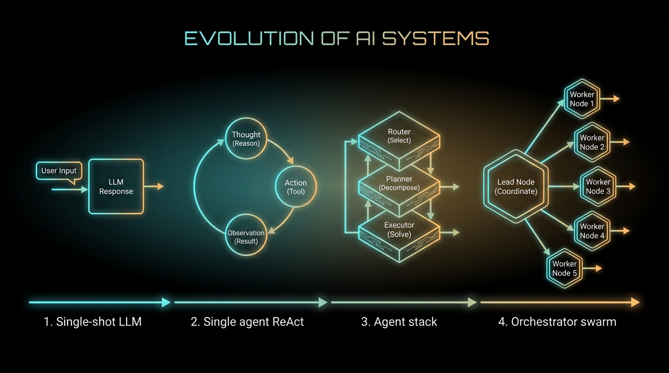
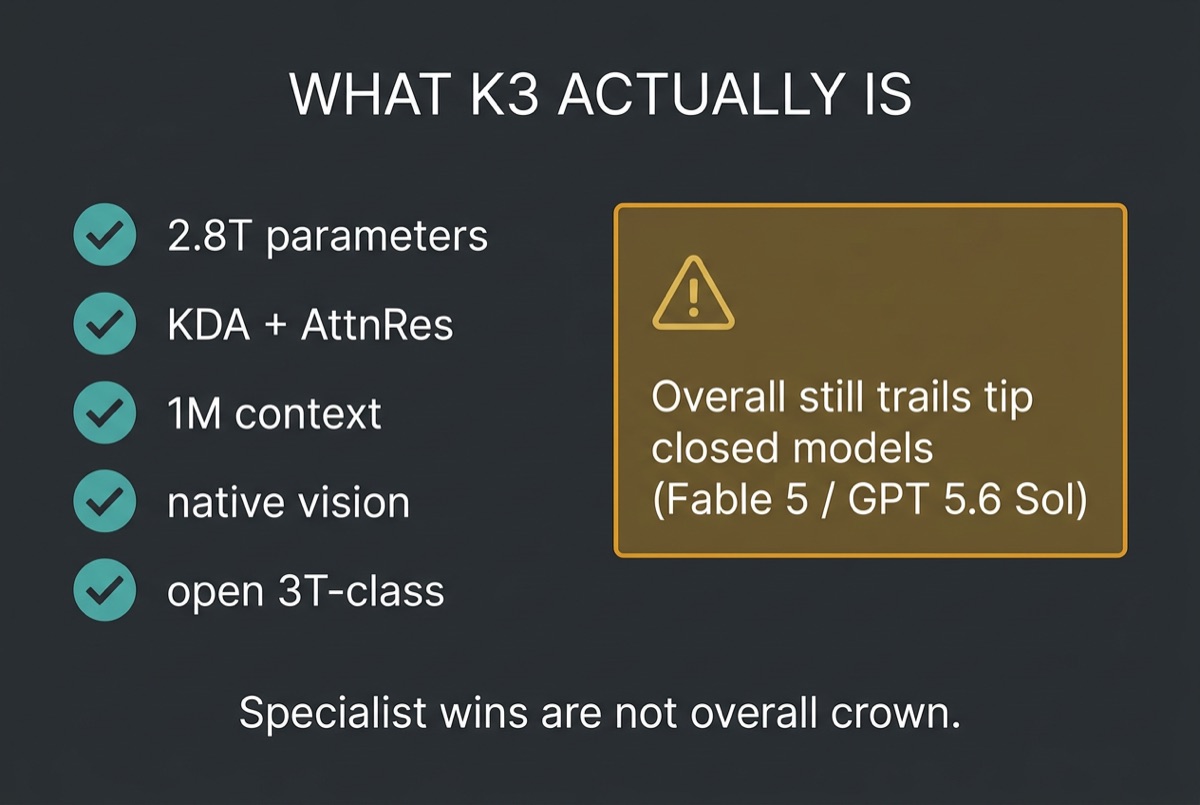
The loudest take on Moonshot’s Kimi K3 is that open weights just “crushed” every closed frontier model. That is marketing gravity, not the lab’s own claim. Treat K3 as what it is: a 2.8-trillion-parameter open 3T-class model with a 1M-token window, native vision, and long-horizon agent strength, that still trails the tip of the closed pack on overall performance, whilst beating it on enough specialised suites that a single-model default is now the expensive mistake.

Lecture map: evaluate, price per task, route, preserve thinking history, planner plus worker — The operating loop for K3: measure the task, price the trajectory, route the specialist, keep the thinking trace intact.

What K3 actually is

Open 3T-class · 1M context · native vision · long-horizon coding

Kimi K3 facts: 2.8T parameters, KDA and AttnRes, 1M context, trails tip closed models overall — Facts first: scale and architecture are real; “beats every closed model” is not the vendor line.

Moonshot’s launch post is unusually honest for a frontier drop. K3 is built on Kimi Delta Attention (KDA) and Attention Residuals (AttnRes), activates 16 of 896 experts under Stable LatentMoE, and is framed for long-horizon coding, knowledge work, and reasoning. Full weights were scheduled for 27 July 2026. Official API pricing at launch: $0.30/MTok cache-hit input, $3.00/MTok cache-miss input, $15.00/MTok output, with Moonshot claiming above 90% cache hit rates on coding workloads.

“While its overall performance still trails the most powerful proprietary models, Claude Fable 5 and GPT 5.6 Sol, Kimi K3 demonstrated frontier-level performance across our evaluation suite, consistently outperforming other tested models.” – Moonshot AI, Kimi K3 tech blog

Hold that sentence against the social-media version. Trails the tip. Outperforms the rest of the tested field. Specialist leaderboards (frontend arenas, terminal suites, legal-agent sets) can still put an open model first without rewriting the overall ranking. If your strategy needs “open crushed closed forever”, you will over-commit. If your strategy needs “open is finally good enough that routing becomes the product”, K3 is the proof point.

Merits of the argument. The open 3T-class framing and the long-horizon coding demos (kernel work, compiler construction, vision-in-the-loop frontend) are load-bearing and primary-sourced. The geopolitics story and the “first open model to dominate every closed model” story are not. Prefer the lab’s caveat over the thumbnail.

Sticker price is a trap; cost per task is the metric

Cache hits · turns · tokens · wall-clock

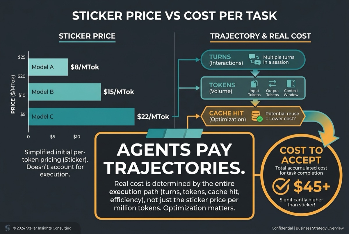
Cost per task diagram comparing sticker dollars per million tokens versus trajectory cost — Same task, different trajectory length: $/MTok lies; cost-to-correct-answer does not.

Everyone quotes input and output rates. Agents do not pay rates; they pay trajectories. A mid-tier model that needs three retries, fifty tool turns, and a bloated context can outspend a flagship that finishes in one disciplined loop. Fireworks’ K3-versus-Fable study makes this concrete: on SWE-style work, K3 often burned far more turns and tokens than Fable, yet still landed cheaper once prompt caching kicked in; on long terminal tasks the spiral flipped and Fable was the one that timed out expensive.

Operational rule: instrument cost per accepted task (and turns-to-accept), not only blended $/MTok. Design prompts and tools so the long prefix is stable enough to hit Moonshot’s automatic context cache (their docs note a previous request must exceed 256 prompt tokens before a later request can hit cache). A 10× token read at $0.30 cache-hit can beat a “cheaper” model that never caches.

Merits of the argument. Cost-per-task is the right unit for agent economics; Kleppmann-style systems thinking applies: measure the path, not the component. Weak point: vendor cache-hit rates are workload-specific. Re-measure on your harness before you rewrite finance slides.

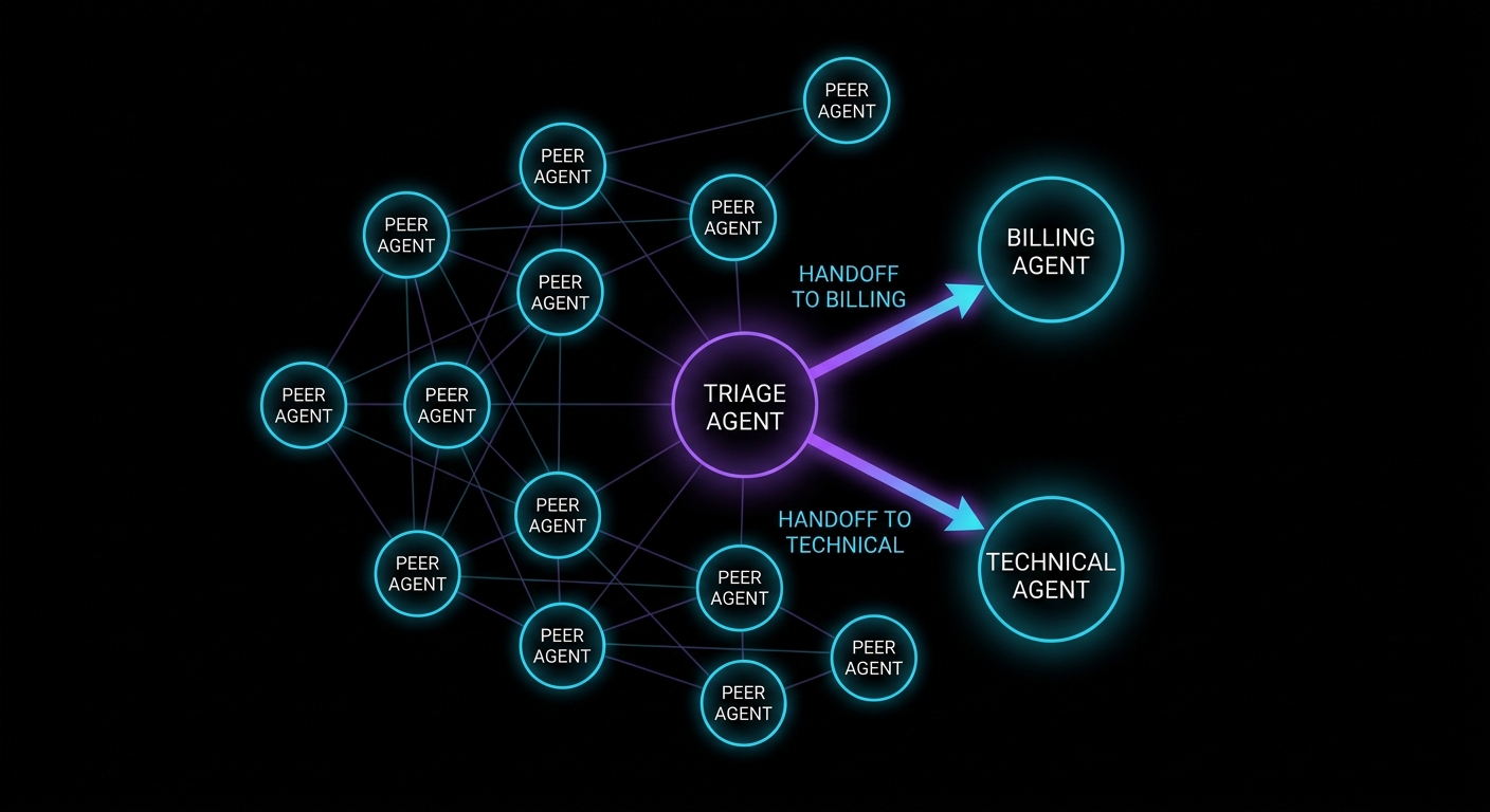
Do not pick a model; route

Specialists · oracle ceiling · production router

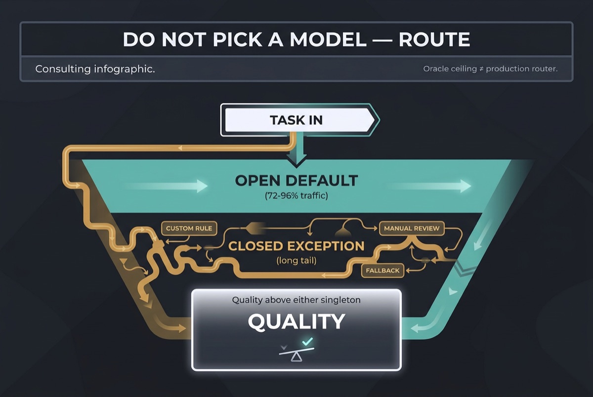
Routing chart: open model default, premium closed model for long-tail tasks — Open as default, closed as exception: quality above either singleton when the router is honest about its ceiling.

Fireworks ran Kimi K3 and Claude Fable 5 through the same agent harness on about 1,030 tasks across SWE, terminal, algorithmic, multi-language, and legal families. Top-line solve rates looked near-tied. Under the hood they specialised: K3 took more of the security, crypto, and long terminal cluster; Fable kept breadth on multi-language and web/data-visualisation slices. Per-task routing beat either model alone.

“We achieved 93% accuracy with routing between K3 and Fable.” – Fireworks AI, Kimi K3 vs Fable study

Read the fine print they published in the same post. Their headline routing figure is driven by oracle routing: run both models, keep the cheapest correct answer. That is a performance ceiling, not a shipped classifier. Oracle traffic still sent 72-96% of tasks to K3 depending on family, which is the strategic signal: open as the default lane, closed as the long-tail exception. Fireworks also sells inference, so treat the cost multiples as directional and rebuild the router on your own eval set (the same discipline we argued in Stop Sending Every Prompt to Your Flagship Model).

Merits of the argument. Specialist complementarity is real and more useful than fan wars. The 93% figure is not a production SLA until you have a router that predicts without double-running. Build that router; do not cosplay it.

Architecture that matters (and claims that do not)

KDA · AttnRes · MoE sparsity · what not to quote

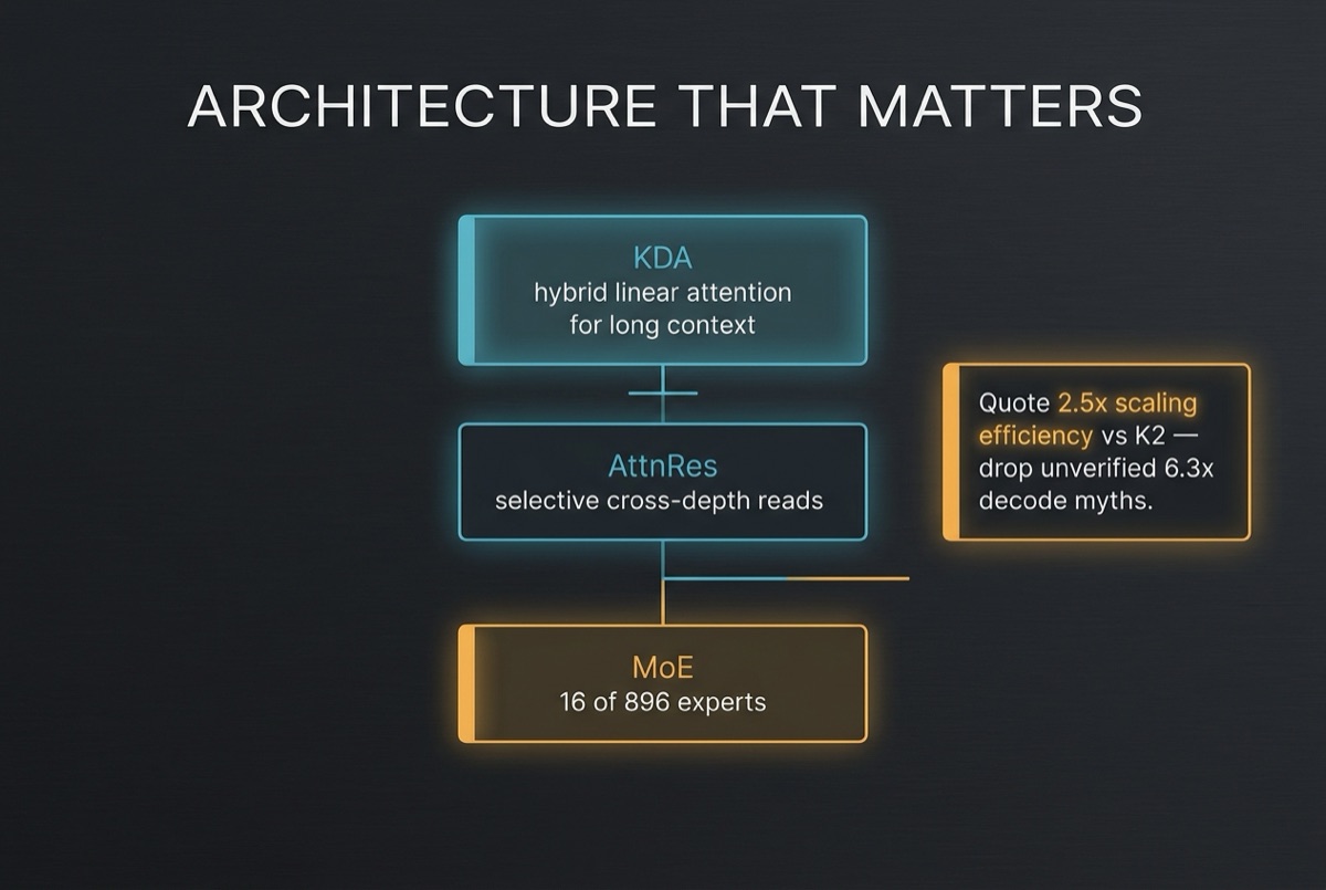
Architecture slide: Kimi Delta Attention, Attention Residuals, 16 of 896 experts — Use the lab’s architecture story; drop viral multipliers that belong to other product tiers.

Two mechanisms are primary-sourced for K3. KDA is Moonshot’s hybrid linear-attention path for long sequences. AttnRes lets deeper layers attend selectively to earlier layer states instead of drowning every insight in one shared residual soup. Combined with aggressive MoE sparsity (16 active of 896), Moonshot reports roughly 2.5× overall scaling efficiency versus Kimi K2. That is the quoteable engineering story.

What does not survive a source check: a precise “6.3× faster decode at 1M tokens because of KDA” line circulating in explainers. Moonshot’s K3 post does not state that figure. A separate ~5-6× throughput claim appears around Kimi Code’s HighSpeed tier on the K2.7 coding stack, which is a product speed tier, not a K3 architecture footnote. Likewise, tidy “plus 25% effective compute for under 2% latency” AttnRes soundbites need a paper citation before they become lecture truth; stick to the published 2.5× scaling-efficiency claim until the technical report lands.

Merits of the argument. Architecture explainers help operators decide when long context and overnight agent loops are the point. Invented multipliers destroy trust. If you cannot grep it on the lab page, paraphrase or cut.

Harness rules that silently break K3

Thinking history · reasoning effort · OpenAI-compatible API · approvals

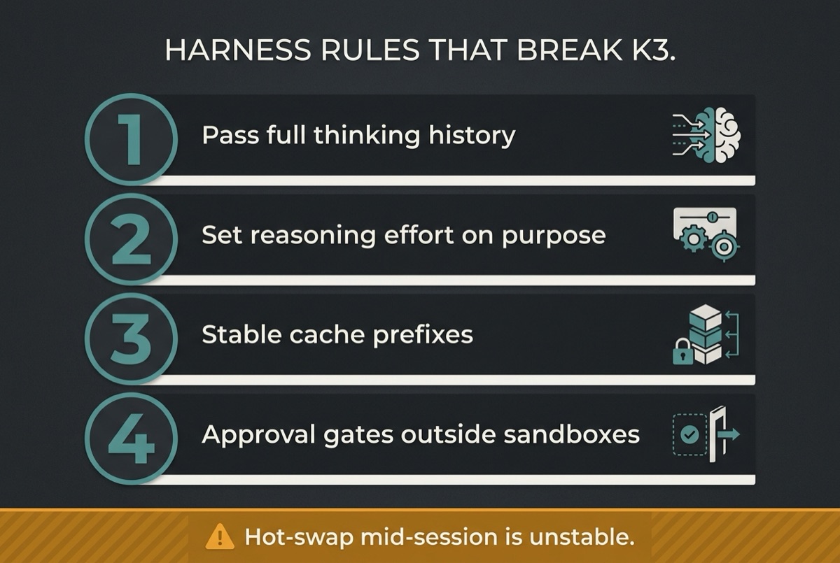
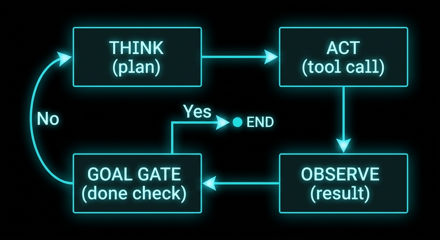
Harness checklist: pass full thinking history, set reasoning effort, stable cache prefix, approval gates — Most “K3 is flaky” reports are harness bugs wearing a model costume.

K3 is not a drop-in chatbot personality you can hot-swap mid-thread. Moonshot trained it with preserved thinking history. If your agent framework strips reasoning_content, truncates assistant messages, or switches into K3 halfway through a session started on another model, quality can collapse without a clean error.

“K3 was trained in the preserved thinking history mode. If the agent harness fails to pass back all the historical thinking content as required, or if an ongoing session with another model is switched over to K3, generation quality may become highly unstable.” – Moonshot AI, Kimi K3 limitations

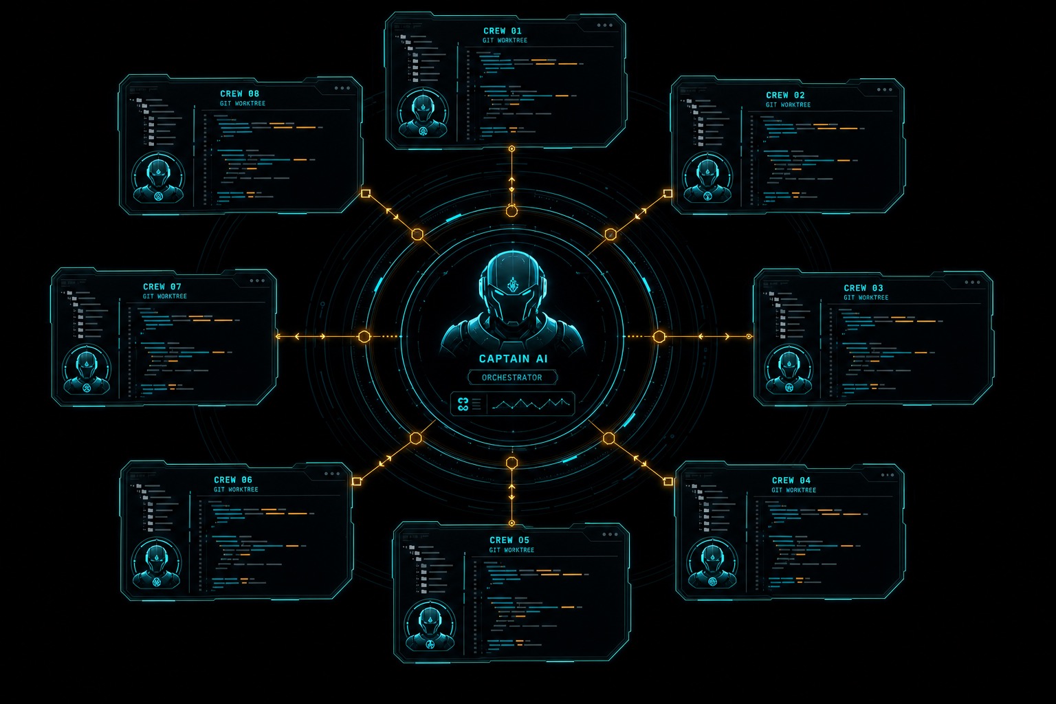
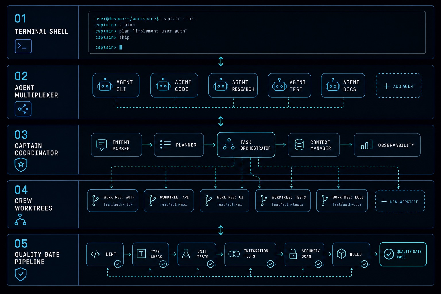
API reality check from the official quickstart: model id kimi-k3, OpenAI-compatible client against Moonshot’s base URL, thinking always on, reasoning_effort of low / high / max (default max at launch). Max effort on trivia is how you set money on fire. Low effort on a multi-hour repo migration is how you get confident wrongness. First-party Kimi Code is the compatibility reference; third-party harnesses (Claude Code, Codex, Pi, custom loops) need an explicit “full assistant message round-trip” test before you trust overnight runs. Pair that with the agent-ops hygiene from Talk to One Agent, Ship With a Crew: one captain surface, gated merges, no YOLO on production trees.

Moonshot also warns about excessive proactiveness: on ambiguous intent, K3 may invent a plan and execute it. That is a feature for long-horizon demos and a liability for regulated repos. Put behavioural fences in system prompts or AGENTS.md when the blast radius is real.

Case 1: Stripped thinking history

A proxy keeps only final content to “save tokens”. Multi-turn tool use drifts, then hallucinates file paths that never existed. Fix: persist and resend the complete assistant message, including reasoning fields, exactly as returned.

Case 2: Max effort for every prompt

Status updates, renames, and one-line shell questions run at max. Bills look like a research lab; latency feels like dial-up. Fix: default high or low for interactive crumbs; reserve max for planned agent jobs with a budget.

Case 3: Single-model religion

All traffic to K3 because the open narrative feels righteous, or all traffic to Fable because the brand feels safe. You pay the specialist tax either way. Fix: route by task family on a frozen eval set; keep a closed model for the long tail your open default fails.

Merits of the argument. The thinking-history constraint is an official footgun, not folklore. Effort knobs and approval gates are boring and they are what separate demos from operations.

Planner plus worker, not flagship for every keystroke

Slow brain · fast hands · overnight loops

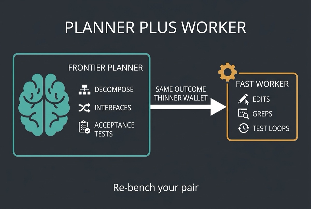
Planner worker pattern: K3 plans, smaller model executes tool steps — Large model writes the plan; small model burns the turns. Same outcome, thinner wallet.

A recurring efficient pattern: use K3 (or another frontier planner) to decompose, choose interfaces, and set acceptance tests; use a cheaper coding model for mechanical edits, greps, and test loops. Pre-K3 team experiments (for example multi-agent SQLite rebuilds from a long manual) already showed near-order-of-magnitude savings when a premium planner rode on a fast worker. Treat those numbers as a pattern, not a K3-specific guarantee. Re-bench with your planner/worker pair.

Self-hosting honesty: 2.8T-class weights will not fit on a laptop. Usable interactive tokens-per-second on a dense or sparsely activated giant wants a serious GPU island; overnight batch on owned hardware is a different economic story. The strategic win of open weights is multi-provider inference and the option to internalise later, not cosplaying a hyperscaler in your spare bedroom. Skip the conspiracy timeline; download when weights are actually published, verify checksums, and decide cloud versus self-host with a spreadsheet, not a meme. And if you do internalise: treat security as a first-class bill of materials, not an afterthought bolted on when someone finds your inference port on Shodan.

Self-host security: open weights move the perimeter

Auth · network isolation · weight integrity · egress · least privilege · audit

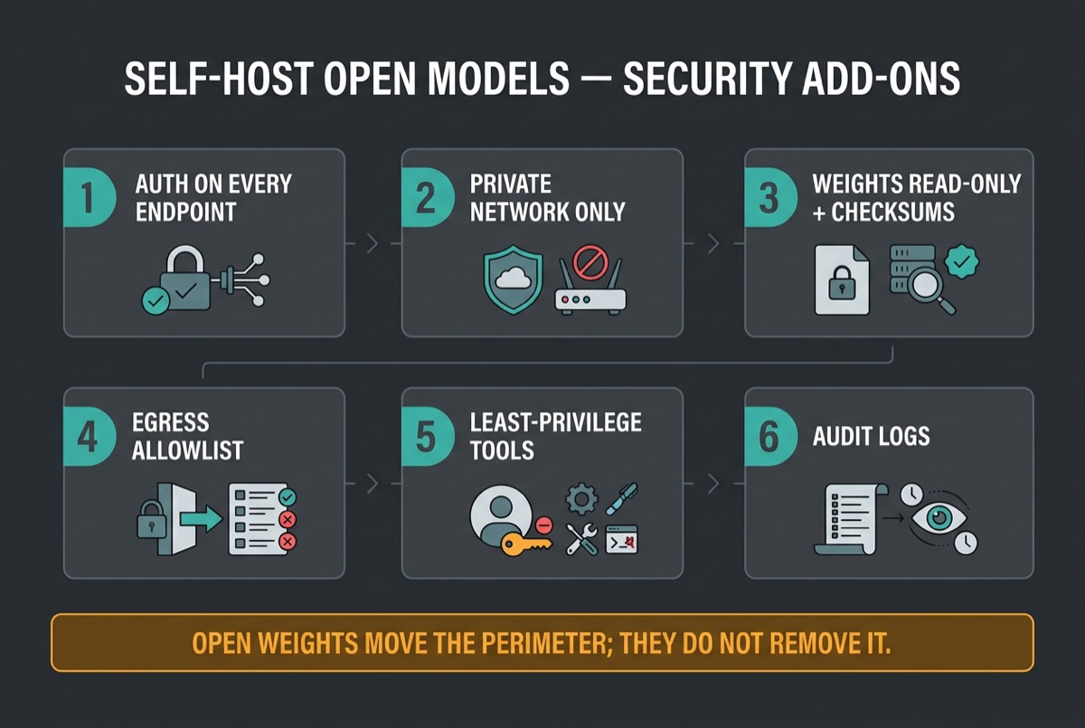
Self-host open models security add-ons: auth, private network, read-only weights, egress allowlist, least-privilege tools, audit logs — Open weights change who runs the GPU. They do not retire the security programme.

Bringing K3 (or any frontier open model) onto your own metal is often sold as “data never leaves”. That is only true if the serving stack, agent tools, and network path are designed that way. An unauthenticated inference endpoint on a GPU box is closer to a public database with no password than to a vault. Self-hosting relocates the trust boundary onto your team; it does not delete prompt injection, tool abuse, supply-chain risk, or silent egress.

“A Prompt Injection Vulnerability occurs when user prompts alter the LLM’s behavior or output in unintended ways.” – OWASP, LLM01:2025 Prompt Injection

For agent harnesses that browse, shell, or call APIs, the blast radius is the tool surface, not the model card. OWASP’s Excessive Agency framing is the right checklist: too many functions, too many permissions, too much autonomy. Moonshot’s own K3 note about unexpected decisions on ambiguous intent is the same class of risk wearing a product-limitation label. On-prem does not make that safer unless you shrink agency in code.

“Excessive Agency is the vulnerability that enables damaging actions to be performed in response to unexpected, ambiguous or manipulated outputs from an LLM, regardless of what is causing the LLM to malfunction.” – OWASP, LLM06:2025 Excessive Agency

Output filters are not enough. Recent agent research on “silent egress” shows a malicious page can induce outbound requests that exfiltrate runtime context while the final answer still looks helpful. Prompt-layer defences helped little; domain allowlisting and redirect-chain controls helped more. If your self-hosted agent can fetch arbitrary URLs, assume the web can talk back as instructions.

“These findings suggest that network egress should be treated as a first-class security outcome in agentic LLM systems.” – Lan et al., Silent Egress (arXiv:2602.22450)

Minimum security add-ons before you put private corpora next to a self-hosted K3:

Auth on every inference endpoint – mutual TLS or gateway JWT/API keys; no bare 0.0.0.0:8000 on a GPU host.
Private network only – inference in a VPC/VLAN with no public ingress; jump hosts or mesh for operators.
Weight supply chain – download from a pinned source, verify checksums/signatures, store on encrypted volumes, mount read-only into the serving container, non-root runtime.
Egress allowlist – default-deny outbound from the agent and tool runners; allow only the registries, package mirrors, and APIs you intend. Log every deny.
Least-privilege tools – no open shell or unbounded web_fetch in production; granular tools, user-scoped credentials, human approval for write/delete/send.
Audit everything – immutable logs of prompts, tool calls, destinations, and approval decisions with correlation IDs. You cannot prove “data stayed local” without them.
Separate planes – keep the chat UI, the model server, and tool executors on different trust zones; never share a host with production secrets “for convenience”.

Case 4: GPU box as public chatbot

Someone exposes vLLM or a similar server to the internet “just for the team”, with no auth. Within days you get scrapers, token burn, and a prompt-injection campaign against whatever tools you later wire in. Fix: bind to localhost or a private interface, put a reverse proxy with auth and rate limits in front, and treat the model port like a database port.

Case 5: Agent with world egress and company docs

Self-hosted model plus RAG over contracts, plus unrestricted HTTP tools. A poisoned PDF or URL preview instructs the agent to POST excerpts to an external host. The UI answer stays polite. Fix: allowlist egress, sandbox retrieval, strip active content from ingested docs, and require approval for any outbound tool that can carry document text.

Merits of the argument. Sovereignty and cost can justify self-hosting. Security is not free with the weights. The controls above are classical systems security applied to an LLM that can act; skip them and you have bought a louder attack surface with a nicer story.

When this is actually fine

Stay on a single closed flagship if your volume is tiny, your eval set is empty, and one vendor’s harness already passes your compliance review. Stay off K3 mid-session hot-swaps until your framework proves thinking-history fidelity. Skip self-hosting until you have a utilisation plan that beats API cache-hit pricing and you can staff the security add-ons above (auth, private network, weight integrity, egress allowlist, least-privilege tools, audit). And do not force K3 onto short interactive Q&A where a small model finishes before K3 finishes “thinking”.

How to get there from here

Stand up the official API with model kimi-k3; confirm multi-turn tool calls resend full assistant messages.
Run a 30-50 task frozen eval across your real work (frontend, backend, terminal, docs, legal-ish review if you do that).
Log cost per accepted task and turns-to-accept for K3 versus your current default.
Add a dumb router: keyword/domain rules first, learned classifier later. Open default, closed exception.
Wire planner/worker for long jobs; keep interactive crumbs on low effort or a smaller model.
Only then consider weight downloads and private inference, with a capacity plan and an exit test against the API baseline.
Before any private corpus touches that stack: auth + private network + checksummed read-only weights + default-deny egress + approval-gated tools + immutable audit logs.

What to check right now

Harness fidelity – Does every tool turn round-trip complete thinking history for K3?
Effort policy – Is max reserved for jobs with a budget, not Slack-style questions?
Cache shape – Are system prompts and retrieved corpora stable prefixes, or rewritten every turn?
Router truth – Do you have a frozen eval, or are you narrating oracle results as production?
Approval gates – Are write/exec tools gated outside disposable sandboxes?
Vendor caveat – Are you quoting “trails Fable 5 / GPT 5.6 Sol overall” instead of “crushed every closed model”?
Self-host auth – Is every inference port behind authentication, or still a bare bind on a GPU host?
Egress policy – Can the agent POST to arbitrary hosts, or is outbound allowlisted and logged?
Weight integrity – Were checksums verified, and are weights mounted read-only?

nJoy 😉

Older posts →